ASTM D2520-21

• Abstract:

  SIGNIFICANCE AND USE; 4.1 Design calculations for such components as transmission lines, antennas, radomes, resonators, phase shifters, etc., require knowledge of values of complex permittivity at operating frequencies. The related microwave measurements substitute distributed field techniques for low-frequency lumped-circuit impedance techniques. ; 4.2 Further information on the significance of permittivity is contained in Test Methods D150. ; 4.3 These test methods are useful for specification acceptance, service evaluation, manufacturing control, and research and development of ceramics, glasses, and organic dielectric materials.; SCOPE; 1.1 These test methods cover the determination of relative (Note 1) complex permittivity (dielectric constant and dissipation factor) of nonmagnetic solid dielectric materials. ; Note 1: The word “relative” is often omitted. ; 1.1.1 Test Method A is for specimens precisely formed to the inside dimension of a waveguide. ; 1.1.2 Test Method B is for specimens of specified geometry that occupy a very small portion of the space inside a resonant cavity. ; 1.1.3 Test Method C uses a resonant cavity with fewer restrictions on specimen size, geometry, and placement than Test Methods A and B. ; 1.2 Although these test methods are used over the microwave frequency spectrum from around 0.5 to 50.0 GHz, each octave increase usually requires a different generator and a smaller test waveguide or resonant cavity. ; 1.3 Tests at elevated temperatures are made using special high-temperature waveguide and resonant cavities. ; 1.4 The values stated in SI units are to be regarded as standard. The values given in parentheses after SI units are inch-pound units that are provided for information only and are not considered standard. ; 1.5 This standard does not purport to address all of the safety concerns, if any, associated with its use. It is the responsibility of the user of this standard to establish appropriate safety, health, and environmental practices and determine the applicability of regulatory limitations prior to use. ; 1.6 This international standard was developed in accordance with internationally recognized principles on standardization established in the Decision on Principles for the Development of International Standards, Guides and Recommendations issued by the World Trade Organization Technical Barriers to Trade (TBT) Committee.

• Status: Published
• Publication Date: 31-Mar-2021
• ICS: 29.035.01 - Insulating materials in general
• Technical Committee: D09 - Electrical and Electronic Insulating Materials
• Drafting Committee: D09.12 - Electrical Tests

• Refers: ASTM D1711-24 - Standard Terminology Relating to Electrical Insulation
• Effective Date: 01-Mar-2024
• Refers: ASTM D1711-15 - Standard Terminology Relating to Electrical Insulation
• Effective Date: 01-Nov-2015
• Refers: ASTM D1711-14a - Standard Terminology Relating to Electrical Insulation
• Effective Date: 01-Nov-2014
• Refers: ASTM D1711-14 - Standard Terminology Relating to Electrical Insulation
• Effective Date: 01-May-2014
• Refers: ASTM D1711-13 - Standard Terminology Relating to Electrical Insulation
• Effective Date: 01-Nov-2013
• Refers: ASTM D1711-11a - Standard Terminology Relating to Electrical Insulation
• Effective Date: 01-Aug-2011
• Refers: ASTM D1711-08 - Standard Terminology Relating to Electrical Insulation
• Effective Date: 01-May-2008
• Refers: ASTM A893/A893M-03(2008) - Standard Test Method for Complex Dielectric Constant of Nonmetallic Magnetic Materials at Microwave Frequencies
• Effective Date: 01-May-2008
• Refers: ASTM D150-98(2004) - Standard Test Methods for AC Loss Characteristics and Permittivity (Dielectric Constant) of Solid Electrical Insulation
• Effective Date: 01-Mar-2004
• Refers: ASTM A893/A893M-03 - Standard Test Method for Complex Dielectric Constant of Nonmetallic Magnetic Materials at Microwave Frequencies
• Effective Date: 01-Oct-2003
• Refers: ASTM D1711-02 - Standard Terminology Relating to Electrical Insulation
• Effective Date: 10-Mar-2002
• Refers: ASTM D1711-99 - Standard Terminology Relating to Electrical Insulation
• Effective Date: 10-Oct-1999
• Refers: ASTM D150-98 - Standard Test Methods for AC Loss Characteristics and Permittivity (Dielectric Constant) of Solid Electrical Insulation
• Effective Date: 10-Feb-1998

Overview

ASTM D2520-21 specifies standard test methods for determining the complex permittivity (dielectric constant and dissipation factor) of nonmagnetic solid electrical insulating materials at microwave frequencies and temperatures up to 1650 °C. Developed by ASTM International, this standard is widely used to evaluate and control the electrical properties of ceramics, glasses, and organic dielectric materials necessary in the design and manufacture of electronic components operating at high frequencies.

Complex permittivity is a critical parameter in applications involving transmission lines, antennas, resonators, phase shifters, and radomes. Accurate measurement at operating frequencies ensures reliable design calculations and helps manufacturers maintain quality, assess service performance, and advance research and development in high-frequency and high-temperature environments.

Key Topics

• Test Methods: ASTM D2520-21 details three principal test methods for measuring complex permittivity over the 0.5 to 50.0 GHz range:

  • Method A: For specimens precisely formed to fit the inside dimension of a waveguide.
  • Method B: For small geometry specimens occupying a minimal portion of a resonant cavity.
  • Method C: Utilizes a resonant cavity with fewer restrictions on specimen size, geometry, and placement.

• High-Frequency and High-Temperature Testing: The standard describes procedures and equipment necessary for microwave measurements at elevated temperatures, using specialized waveguides and cavities to withstand environmental stresses up to 1650 °C.

• Measurement Parameters: Focus is placed on:

  • Dielectric constant (κ'): Real part of permittivity, critical to energy storage in a material.
  • Dissipation factor (tan δ): Indicates energy loss, important for assessing material efficiency.

• Distributed Field Techniques: Microwave permittivity measurements leverage distributed field techniques, in contrast to traditional low-frequency lumped-circuit approaches.

Applications

ASTM D2520-21 is indispensable for a range of practical scenarios including:

• Product Design and Engineering: Enables precise calculation of component behaviors such as signal speed, loss, and efficiency in transmission lines, antennas, radomes, and resonators at microwave frequencies.
• Specification and Quality Control: Used for material specification acceptance and process control in manufacturing, especially vital for industries such as telecommunications, aerospace, and electronics.
• Service Evaluation: Supports assessment of materials under operational conditions matching real-world high-frequency and high-temperature environments.
• Research and Development: Facilitates the exploration and optimization of new dielectric materials, including ceramics, glasses, and organic alternatives, especially for advanced RF and microwave systems.

Related Standards

• ASTM D150: Test Methods for AC Loss Characteristics and Permittivity (Dielectric Constant) of Solid Electrical Insulation. Addresses permittivity at lower frequencies.
• ASTM A893/A893M: Test Method for complex dielectric constant of nonmetallic magnetic materials at microwave frequencies-complements D2520 by covering magnetic materials.
• ASTM D1711: Terminology Relating to Electrical Insulation. Provides definitions and terminology referenced throughout D2520.

These referenced standards collectively provide a comprehensive framework for evaluating and comparing the dielectric properties of insulating materials across a broad frequency and environmental range.

---

Keywords: ASTM D2520, dielectric constant measurement, complex permittivity, microwave frequencies, insulating materials, dissipation factor, high temperature, quality control, electronics, transmission lines, antennas, radomes, resonators, material testing standard.

This international standard was developed in accordance with internationally recognized principles on standardization established in the Decision on Principles for the
Development of International Standards, Guides and Recommendations issued by the World Trade Organization Technical Barriers to Trade (TBT) Committee.
Designation: D2520 − 21
Standard Test Methods for
Complex Permittivity (Dielectric Constant) of Solid Electrical
Insulating Materials at Microwave Frequencies and
Temperatures to 1650 °C
This standard is issued under the fixed designation D2520; the number immediately following the designation indicates the year of
original adoption or, in the case of revision, the year of last revision.Anumber in parentheses indicates the year of last reapproval.A
superscript epsilon (´) indicates an editorial change since the last revision or reapproval.
1. Scope mendations issued by the World Trade Organization Technical
Barriers to Trade (TBT) Committee.
1.1 These test methods cover the determination of relative
(Note 1) complex permittivity (dielectric constant and dissipa-
2. Referenced Documents
tion factor) of nonmagnetic solid dielectric materials.
2.1 ASTM Standards:
NOTE 1—The word “relative” is often omitted.
A893/A893MTest Method for Complex Dielectric Constant
1.1.1 TestMethodAisforspecimenspreciselyformedtothe
of Nonmetallic Magnetic Materials at Microwave Fre-
inside dimension of a waveguide.
quencies
1.1.2 Test Method B is for specimens of specified geometry
D150Test Methods forAC Loss Characteristics and Permit-
that occupy a very small portion of the space inside a resonant
tivity (Dielectric Constant) of Solid Electrical Insulation
cavity.
D1711Terminology Relating to Electrical Insulation
1.1.3 Test Method C uses a resonant cavity with fewer
restrictions on specimen size, geometry, and placement than
3. Terminology
Test Methods A and B.
3.1 Definitions:
1.2 Although these test methods are used over the micro-
3.1.1 For definitions of terms used in this test method, refer
wave frequency spectrum from around 0.5 to 50.0 GHz, each
to Terminology D1711.
octave increase usually requires a different generator and a
3.2 Definitions of Terms Specific to This Standard:
smaller test waveguide or resonant cavity.
3.2.1 neper, n—a division of the logarithmic scale wherein
the number of nepers is equal to the natural logarithm of the
1.3 Tests at elevated temperatures are made using special
scalar ratio of either two voltages or two currents.
high-temperature waveguide and resonant cavities.
NOTE 2—The neper is a dimensionless unit. 1 neper equals 0.8686 bel.
1.4 The values stated in SI units are to be regarded as
With I and I denoting the scalar values of two currents and n being the
standard. The values given in parentheses after SI units are x y
number of nepers denoted by their scalar ratio, then:
inch-poundunitsthatareprovidedforinformationonlyandare
not considered standard.
n 5ln ~l ⁄ l !
e x y
1.5 This standard does not purport to address all of the
where:
safety concerns, if any, associated with its use. It is the
ln = logarithm to base e.
e
responsibility of the user of this standard to establish appro-
3.3 Definitions of Terms Specific to Test Methods B and C:
priate safety, health, and environmental practices and deter-
3.3.1 electrical skin depth, n—the effective depth of field
mine the applicability of regulatory limitations prior to use.
penetration at high frequencies where electric currents are
1.6 This international standard was developed in accor-
confinedtoathinlayeratthesurfaceofconductorsduetobasic
dance with internationally recognized principles on standard-
electromagnetic phenomena.
ization established in the Decision on Principles for the
3.3.1.1 Discussion—The skin depth for copper and silver is
Development of International Standards, Guides and Recom-
approximately0.002mmat1GHzanddecreasesbyafactorof
10 at 100GHz.
These test methods are under the jurisdiction of ASTM Committee D09 on
Electrical and Electronic Insulating Materials and is the direct responsibility of
Subcommittee D09.12 on Electrical Tests. For referenced ASTM standards, visit the ASTM website, www.astm.org, or
Current edition approved April 1, 2021. Published June 2021. Originally contact ASTM Customer Service at [e-mail]. For Annual Book of ASTM
approved in 1966. Last previous edition approved in 2013 as D2520–13. DOI: Standards volume information, refer to the standard’s Document Summary page on
10.1520/D2520-21. the ASTM website.
Copyright © ASTM International, 100 Barr Harbor Drive, PO Box C700, West Conshohocken, PA 19428-2959. United States
D2520 − 21
3.3.2 high Q cavity, n—a rectangular cavity having a Q able. Transmission lines capable of withstanding temperatures
greater than 2000. up to 1650°C in an oxidizing atmosphere can be used to hold
3.3.2.1 Discussion—Q defines the bandwidth (or sharpness) the specimen.
of the resonance curve of field intensity plotted against
6. Summary of Test Method
frequency. Q is the reciprocal of the electrical loss with a high
6.1 For an isotropic dielectric medium, one of Maxwell’s
Q indicating low electrical losses of the cavity and dielectrics
curl equations is written:
and is obtained by optimum choice of cavity dimensions, use
of high conductivity metals (such as silver and copper) with
curl H 5 jωκ*ε E (1)
highly polished surfaces (that is, surface roughness much
assuming exp (jωt) time dependence, where:
smallerthanelectricalskindepthatthetestfrequency).HighQ
κ* = relative complex permittivity,
is enhanced by choice of large cavity volume to surface area.
ε = (absolute) permittivity of free space, and
Surface irregularities or variations in flatness, radius of
ω =2πf, f being the frequency.
curvature, or parallelism of walls, leads to spurious resonance
The notation used will be as follows:
modes which introduce electrical losses and lower the cavity
Q.
κ* 5 κ'2jκ" 5 κ' 1 2 j tan δ (2)
~ !
3.3.3 microwave, adj—referring to electromagnetic wave-
where:
lengths of 30cm or less where the corresponding frequency is
tan δ = κ"/κ',
1GHz or higher.
κ' = real part, and
3.3.4 resonant cavity, n—an enclosure with conducting
κ" = imaginary part.
walls which will support electromagnetic resonance of various
Thevalueof κ*isobtainablefromobservationsthatevaluate
specific modes dependent on the cavity geometry and
theattenuationandwavelengthofelectromagneticwavepropa-
dimensions,andontheintegralnumberofhalfwavesandtheir
gation in the medium.
directions of propagation as terminated by the cavity walls.
6.2 The permittivity of the medium in a transmission line
3.3.4.1 Discussion—In practice, allowance must be made
affects the wave propagation in that line. Obtain the dielectric
forinputandoutputcouplingholes,probes,orloops.Openings
properties of a specimen by using a suitable line as a dielectric
or means of disassembling must be provided for introducing
specimen holder. The electromagnetic field traveling in one
dielectric specimens.
directioninauniformlinevarieswithtime,t,andwithdistance
along the line, χ, as exp (jωt 6 γχ) where γ is the propagation
4. Significance and Use
constant.Assumingthatthemetalwallsofthelinehaveinfinite
4.1 Design calculations for such components as transmis- conductivity the propagation constant γ of any uniform line in
sion lines, antennas, radomes, resonators, phase shifters, etc.,
a certain mode is:
require knowledge of values of complex permittivity at oper-
22 22 1⁄2
γ 5 2π λ 2 κ * λ (3)
~ !
c
ating frequencies. The related microwave measurements sub-
where:
stitute distributed field techniques for low-frequency lumped-
circuit impedance techniques.
λ = cut-off wavelength for the cross section and the
c
mode in question,
4.2 Furtherinformationonthesignificanceofpermittivityis
λ(=c⁄f) = wavelength of the radiation in free space, and
contained in Test Methods D150.
κ* = relative complex permittivity of the nonmag-
4.3 These test methods are useful for specification
netic medium.
acceptance, service evaluation, manufacturing control, and
Since κ* is complex, γ is complex, that is:
research and development of ceramics, glasses, and organic
λ 5 α1jβ (4)
dielectric materials.
The field dependence on distance is therefore of the form
TEST METHOD A—SHORTED TRANSMISSION −αχ −jβχ
e e . The wave attenuation is α in nepers per unit length;
LINE METHOD
β is the phase constant, β=2 π⁄λ where λ is the guide
g g
wavelength in the line. The method of observing α and β by
5. Scope
impedancemeasurementsandofrepresentingthebehaviorofa
5.1 Thistestmethodcoversthedeterminationofmicrowave
line containing a dielectric by means of the formalism of
dielectric properties of nonmagnetic isotropic solid dielectric
transmission line impedance will be outlined briefly (1).
materials in a shorted transmission line method. This test
6.3 Impedance Representation of Ideal Problem—The im-
method is useful over a wide range of values of permittivity
pedance representation of the ideal problem is illustrated by
and loss (1). It is suitable for use at any frequency where
Fig. 1 for a uniform line terminated by a short. In Fig. 2 a
suitable transmission lines and measuring equipment are avail-
dielectric specimen of length d is supposed to fill completely
s
the cross section of the line and be in intimate contact with the
3 flat terminating short. The impedance of a dielectric filled line
The boldface numbers in parentheses refer to the list of references appended to
these test methods. terminated by a short (1), observed at a distance d from the
s
D2520 − 21
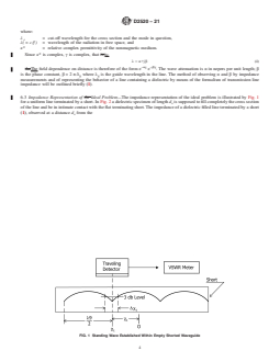
FIG. 1 Standing Wave Established Within Empty Shorted Waveguide
FIG. 2 Standing Wave Established Within Shorted Waveguide After Insertion of Specimen
Also refer to Refs (1-4) for information on air gap corrections and use of
short (at what is defined as the input face of the specimen) is:
standard materials to reduce errors and improve accuracy.
Z 5 ~j ω µ ⁄ γ tanh ~γ d !! (5)
in 0 2 2 s
When r is small, a correction is necessary (5). The load
where:
impedance at a phase distance u away from an observed
µ = the permeability of free space and of the material, and electric node having VSWR=r is:
γ = given by Eq 2, using the dimensions of the line around
Z 5 Z ~1 2 jr tan u!⁄~r 2 j tan u! (7)
meas 01
the specimen.
where:
6.4 Impedance Measurement:
Z = jωµ /γ =fµ λ , assuming the line is uniform and
01 0 1 0 g
6.4.1 The object of the measurement is to obtain the
lossless.
impedance at the input face of the specimen for evaluation of
6.4.2 It remains to determine r and u correctly, taking into
theunknown γ inEq4whichinturnallowsK*tobeevaluated
in Eq 2. The impedance in question is measured by a traveling account losses of the line and nonuniformity due to tempera-
ture differences, then to equate Z and Z from Eq 6 and Eq
probe in a slotted section of the line. As illustrated schemati-
meas in
cally in Figs. 1 and 2, the position of an electric node, that is, 4,andfinallytolayoutaconvenientcalculationschemefor κ*.
The measuring procedure for obtaining r and u is discussed in
an interference minimum of the standing wave, is observed,
and also the “width,” ∆χ, of this node is observed. ∆χ is the Section 10.
distancebetweentwoprobepositionsoneithersideofthenode
7. Significance and Use
position where the power meter indicates twice the power
existingatthenodeminimum.Thevoltagestandingwaveratio
7.1 This test method is useful for quality control and
denoted by r (r =VSWR) is obtained from ∆χ by the equation acceptancetestsofdielectricmaterialsintendedforapplication
(see λ , Section 11):
at room and substantially higher temperatures. Dielectric
gs
measurement capabilities over wide ranges of temperature and
r 5 λ⁄π∆χ (6)
over wide, continuous ranges of frequency provide significant
NOTE 3—Refer to Appendix X2 and Appendix X3 for additional
comments on errors and refinements in the method to improve accuracy. usefulness of this method for research and development work.
D2520 − 21
8. Apparatus 8.2 The so-called slope of the attenuation characteristic of
the slotted line is to be normal, that is, the VSWR is changing
8.1 See Fig. 3 for a block diagram of equipment compo-
by the expected amount in going from one node to another
nents.Somecharacteristicsofthecomponentineachblockare
while looking into a shorted termination. Items 8.1.5, 8.1.8,
as follows:
and 8.1.10 shall have initial dimensions plus differential
8.1.1 Generator—Stable in power and frequency with low
expansions at the temperature of a junction so that the change
harmonic output.
in dimensions is less than 0.25 mm (0.01 in.). The dielectric
8.1.2 Square-Wave Modulator—1.0 kHz output or fre-
holdershallslopedownwardat45to90°tomaintainspecimen
quency required for VSWR meter.
against termination. Termination shall be flat to 0.010 mm
8.1.3 Frequency Meter—Heterodyne or cavity absorption;
(0.0004 in.) and perpendicular to axis of waveguide within
uncertainty 1 part in 10 .
60.05°.At9GHz,thetoleranceontransversedimensionsshall
8.1.4 Isolator—30-dB isolation, and having an output
be 60.075 mm (0.003 in.).
VSWR of less than 1.15.
8.1.5 Slotted Section—A slotted waveguide section and
9. Sampling
carriage capable of measuring gross distances to 0.025 mm
−4
9.1 Determine the sampling by the applicable material
(0.001 in.) and small distance to 0.0025 mm (10 in.) (for
specification.
node width). A micrometer head is required; it is to move
parallel to the axis of the line.
10. Test Specimen
8.1.6 Probe—Adjustable for depth. The detector must be
10.1 The transverse dimensions of the specimen shall be
square law (6) if one uses the voltage-decibel scale of the
0.05 6 0.025 mm (0.002 6 0.001 in.) less than those of the
standing wave ratio (SWR) meter. The detector must be
transmission line. The front and back faces shall be parallel
operatedinthesquarelawregion.And,inparticular,thecrystal
within 0.01 mm (0.0004 in.) and perpendicular to the axis of
detectors will comply with the square law, if they are not
the transmission line within 60.05°. The corners of the
overdriven. The law of a crystal is checked commonly by
specimen are slightly rounded so the end surface seats flat
adding a good rotating-vane microwave attenuator.
against the termination with no air film between the surfaces.
8.1.7 VSWR Meter—Readable in decibels.
The length, d , shall be suitable for the measurement; a length
8.1.8 Temperature Isolation Section—Includes a bend.
s
of1mm(0.04in.)shallbeusedin1by23mm(0.04by0.9-in.)
8.1.9 Cooling Sink—Sufficient conduction to water or air
rectangular waveguide. For high loss materials the length is
streamtomaintainsuitabletemperatureandwaveguidedimen-
controlledbytheelectricalcriteriongivenforntan δin12.2.2.
sions.
8.1.10 Waveguide Specimen Holder—Platinum-20% rho-
11. Procedure
dium for 1650°C; platinum for temperature 1300°C; copper
or silver for lower temperatures within their abilities to 11.1 Impedance measurements are required in the empty
withstand thermal damage and corrosion. Length shall be line (Fig. 1), and with the specimen in place (Fig. 2). The
sufficienttohaveamaintransitionregionoftemperatureofthe frequency of the source and the temperature distribution of the
orderof λ inextentandstillkeepsampletemperatureuniform linearetobethesameforbothobservations.Withnospecimen
g
to 5°C. (Fig.1)readtheposition χ ofavoltageminimum(anode),on
8.1.11 Tube Furnace—Platinum-wound tube furnace to ac- ascaleofarbitraryorigin;alsomeasuretheseparationbetween
cept test section, and maintain a 50 mm (2-in.) length at a positions either side of χ where the power is+3.01 dB from
constant temperature 65°C up to 1650°C. the minimum. This is the width ∆χ of the node. Likewise
FIG. 3 Block Diagram of Apparatus Used to Perform Measurement of Dielectric Properties by Short Circuit Line Method
D2520 − 21
measure this analogous χ and ∆χ with the specimen against β d tan β d 5 λ ⁄2 π d tan u (13)
~ ! ~ !
2 s 2 s gh s
2 2
the termination (Fig. 2).As an additional check measurement,
From Eq 2, assuming tan δ is small,
in one case measure the distance between two adjacent nodes.
22 22 1⁄2
β 5 2π κ ' λ 2 λ (14)
~ !
2 c
This distance is λ /2, where λ is the guide wavelength in the
gs gs
slotted section.
which gives κ' after β d has been found in Eq 12.
2 s
2 22 22
κ' 5 β⁄2 ⁄2 π 1 λ ⁄λ (15)
@~ ! #
2 c
12. Calculation
Of course, λ is based on the size of the heated waveguide
c
12.1 Measurements Transformed to Input Face of
holder. The other part of Eq 11 gives:
Specimen—When measurements are made at elevated
temperatures, the guide width and the guide wavelength, λ , ∆χ
g
tanδ 5 FG (16)
vary because of the temperature gradient between the heated d
s
section and the cool (room temperature) slotted section. For-
where:
tunately the argument of the tangent in Eq 6 is obtainable,
2 2
F 5 1 2 κ ⁄κ'λ (17)
assuming the change in λ is not abrupt. The correct argument c
g
is:
and:
u 5 2π@N⁄2 2 d ⁄ λ 6 ~χ 2 χ ⁄ λ !# (8) 2
gh 2 1 gs
1 1 tan u
~ !
G 5 (18)
~1 1 tan β d! 2 ~tan β d ⁄ β d!
Where λ is calculated for the empty heated dielectric 2 2 2
gh
holder section from the dimensions duly adjusted for thermal
The paper (7) on separating Eq 12-17 from Eq 11 is to be
expansion. In Eq 7 the plus sign is used if the scale for χ
consulted. The loss tangent in Eq 15 contains a contribution
increases away from the short, the minus sign if the opposite.
from the metal walls around the specimen; corrections are
N is the smallest integer 0, 1, etc., that makes u positive. To
available (2, 7).
calculate λ use the general equation:
gh
12.2.3 Finally, a correction in κ' (at least, and ideally in tan
22 22 22
δ also) is required due to the air gap around the specimen.
λ 5 λ 2 λ (9)
gh c
Theoretical treatment (3, 8, 9) indicates that in rectangular
where:
TE guide:
λ = c/f=free space wavelength, and
b
λ = cutoff wavelength calculated from the dimensions.
c
κ' 5 κ' (19)
Eq13
b 2 ~b 2 b!κ'
w w Eq13
For the TE mode rectangular guide discussed below,
where:
λ =2a*wherea*isthewidedimension.Itremainstofindthe
c
∆χ (width of the node) that would have been measured at the b and b = the shorter cross-sectional dimensions of the
w
face of the specimen. The node width ∆χ without the
specimenandguide,respectively,takingaccount
specimen is assumed to arise from the attenuation factor of the of thermal expansion.
empty line, and can be treated as if it increased smoothly with
Someexperiments (10)disagreewithEq18.Thecalculation
distance from the short. The width contribution accumulated
scheme in Appendix X1 uses experimental corrections.
duetoattenuationingoingfromthesamplefacetotheplace χ
where it is observed is ∆χ (L −d )/L where L is the total 13. Report
1 2 s 1 i
length of path, i =1 or 2, to the shorting termination and d is
s
13.1 Report the following information:
the length of the specimen.The node width ∆χ, transformed to
13.1.1 The unique identity of the material tested, that is,
the sample face is therefore obtained approximately as:
name, grade, color, manufacturer, or other pertinent data,
∆χ 5 ∆χ 2 ∆χ L 2 d ⁄L (10)
~ ! 13.1.2 Test temperature,
2 1 s 1
13.1.3 Dimensionsofspecimenandwaveguideholdercross
A more exact treatment would require knowing the attenu-
section.
ation as a function of distance throughout. In a high tempera-
13.1.4 Thermal expansion coefficient of specimen and
ture holder, with L >> d, use an adequate approximation:
waveguide at each temperature,
∆χ 5 ∆χ 2 ∆χ (11)
2 1 13.1.5 Frequency, f,
13.1.6 χ − χ , and
12.2 Equations to Be Solved:
2 1
13.1.7 Calculated value of κ' and tan δ.
12.2.1 Setting the impedances from Eq 4 and 6 equal gives:
µ µ λ 1 2 jr tan u
~ !
0 0 gh 14. Precision and Bias
tanh γ d 5 (12)
2 s
γ j2π~r 2 j tan u!
14.1 The main sources of error in κ' are from air gaps either
−1
Dividing by d Eq 11 is of the form Z tanh Z equal to a between the specimen and the short or in the direction of the
s
known complex number, where Z = γ d . Solutions can be
electric field. Variations in κ' with the specimen length d and
2 s s
obtained (1) and k* calculated. due to turning it over frequently indicate a termination air gap.
12.2.2 If tan δ is less than 0.1 and n tan δ is less than 0.4, The gap involved in Eq X3.20 is to be carefully evaluated. A
where n is the number of half wave segments contained in the weighted average, weighted by the sine squared across the
specimen, it is a reasonable approximation to separate real and guide, shall be used. Errors in loss arise mainly from imper-
imaginary parts in Eq 11 and obtain (7): fection of the probe coupling and from inability to determine
D2520 − 21
the losses q, ∆χ , and ∆χ. It is helpful to verify the measure- maximum and the magnetic field is zero. Although most
5 t
ment system by measuring the loss of a standard reference dielectric materials have relative permeability of unity, there
material having low loss, especially when κ' is of the order of are materials like ferrites where both relative permittivity and
9 to 10 (see Note 2 in 6.4.1). permeability are greater than unity.
TEST METHOD B—RESONANT CAVITY
19. Apparatus
PERTURBATION METHOD
19.1 Fig. 4 is a sketch of a typical rectangular test cavity,
which is in reality, a short section of rectangular waveguide.
15. Scope
Metallicplatesboltedorsolderedtotheendflangesconvertthe
15.1 This test method covers the measurement of micro-
transmission line into a resonant box.An iris hole in each end
wave complex permittivity of dielectric specimens in the form
plate feeds energy into and out of the cavity. The cavity
of rods, bars, strips, sheets, and spheres. The measurement
electrical losses are to be low, which requires the “Q”tobe
frequency depends on the available resonant modes in a
greater than 2000 (see 15.1). A clearance hole centered in
resonant cavity, which limits freedom of selection to a few
opposite walls is provided so that cylindrical rod or spherical
values of frequency for a given cavity. Resonant cavities
specimenscanbeintroducedintoaregionofmaximumelectric
exhibit very high Q values (2000 to 5000 or more) and are
field. Strip or sheet specimens have to be introduced by
therefore inherently sensitive for low loss measurements. The
removing one of the end walls. A list of apparatus follows:
perturbation method requires that the specimen be relatively
19.2 Microwave Frequency Meter, 6-digit precision.
small compared to the volume of the cavity and that the
specimen must be positioned symmetrically in a region of
19.3 VSWR Meters, or equivalent power indicators, 0.1 dB
maximum electric field. Although resonant cavities are sensi- or less sensitivity.
tive to low loss materials, the small specimen size limits the
19.4 Crystal Diodes and Holders, or bolometers.
precision attainable. Nevertheless, the method has several
19.5 Directional Couplers, or waveguide to coax adaptors.
additional advantages besides reasonably good precision:
15.1.1 Although dimensions are important and must be
NOTE 4—These items cover one band of frequencies only, such as X
measured accurately, the specimen does not have to have a band (8 to 11 GHz).
close tolerance fit within the specimen holder as in Test
19.6 Microwave Signal Generator, adjustable frequency.
Method A.
19.7 Square-Wave Modulator (if VSWR meters used).
15.1.2 The calculations for the perturbation method are
19.8 Variable Attenuator, precision-calibrated, 0.1 dB or
relativelysimple,anddonotrequiredigitalcomputersortables
of complex functions. less uncertainty, range 10 dB or more.
19.9 Variable Attenuator.
15.2 Thespecimenshapesmentionedabovehavebeenused
for ceramics and ferrites as well as homogeneous organic
19.10 Isolators.
materials. The thin strip or sheet is adaptable to laminates.
19.11 Set Waveguide Hardware, coaxial cables, connectors,
etc.
16. Summary of Test Method
19.12 ConventionalVSWRmeterscontainhighgainampli-
16.1 The introduction of a dielectric specimen into a reso-
fiers tuned to 1000 Hz. This requires 1000 Hz modulation.
nant cavity lowers the resonant frequency and lowers the Q of
Digitalfrequencymetersgenerallydonotworkonsquarewave
the cavity. The permittivity and dissipation factor of the
modulatedsignals.A100-MHzdigitalfrequencycounterplusa
specimen can be calculated from measurements of resonant
transfer oscillator are often used by mixing a harmonic of the
frequency and Q of the cavity with and without the specimen,
oscillator with the microwave signal to get a “beat frequency”
andfromcavityandspecimendimensions.Whenthespecimen
null on an oscilloscope. The counter reads fundamental oscil-
is small compared to wavelength, perturbation theory allows
lator frequency, which when multiplied by the number of the
simplification of the calculations.
harmonic, is equal to the microwave frequency. This method
works on either modulated or unmodulated signals.
17. Significance and Use
19.13 Avariation of the above system uses an unmodulated
17.1 This test method is useful for specification acceptance,
signal generator connected to a digital frequency meter, fol-
service evaluation, manufacturing control, and research and
development of ceramics, glasses, and organic dielectric ma- lowed by a crystal diode modulator or equivalent. This allows
the use of sensitive VSWR meters. If modulation is omitted
terials. It has also been widely used for magnetic ferrites as
Test Method A893/A893M. entirely, microwave power meters can be used, but due to
lower sensitivity, a microwave amplifier is necessary to raise
18. Interferences
the power input above noise level.
18.1 Test MethodAis sensitive to magnetic permeability as
19.14 Another approach substitutes a microwave received
well as dielectric permittivity. This test method requires that
heterodyne system instead of square wave modulation and
the relative complex permeability be of unit magnitude. Test
Method B is insensitive to permeability since the specimen is
small and is introduced in a region where the electric field is
D2520 − 21
2 2
Resonant Frequency: f = 15 [(1/W) +(N/d) ] ⁄2 gigahertz.
* h, w, and d are cavity inside dimensions in centimetres.
FIG. 4 Rectangular Microwave Cavity for Permittivity Measurements by Perturbation Method
VSWR meters. This requires an additional tuned microwave several measurements shall be made along the length to check
oscillator, which beats against the signal generator to produce dielectric uniformity. The 1.04 mm (0.041-in.) diameter is
a difference frequency of around 30 MHz, which is then rather small and quite difficult to fabricate. Some laboratories
amplifiedbyatunedI.F.amplifieranddetectortogetasuitable have used specimen diameters as large as 2.03 mm (0.080 in.)
indication on a d-c milliammeter. with a resultant negative error of approximately 2% on
materials with permittivity around 8 to 10. By the use of
19.15 Fig. 5 is a block diagram of a typical microwave
standard specimens, it is possible to introduce corrections
system for the resonant cavity perturbation method.
which will eliminate this error. Rod specimens at S-band
20. Sampling frequencies (2.6 to 3.9 GHz) is to be 3.20+0.00,−0.05 mm
(0.126+0.000,−0.002 in.) in diameter.
20.1 Determine the sampling by the applicable material
21.1.2 Spherical Specimens—The diameter of spherical
specification.
specimens also is to be small (approximately 10% or less)
compared to wavelength.
21. Test Specimen
21.1.3 Strip and Sheet Specimens—The thickness of the
21.1 Dimensions and Tolerances:
strip and sheet specimens also is to be small (10% or less)
21.1.1 Rod Specimens—The optimal diameter of rod speci-
compared to wavelength.
mens at X-band frequencies (8 to 12 GHz) is 1.04 6
0.00,−0.05 mm (0.041+0.000,−0.002 in.). The active length 21.2 Rod specimen diameter is to be measured by microm-
is the inside height of the waveguide cavity, 10.16 mm etertowithin 60.0025mm(0.0001in.)atthreelocationsalong
(0.4in.). However, if the specimen is introduced through holes the active length and at three radial locations around the rod.
in the wall, the specimen length is to be longer than 12.5 mm These measurements are then averaged. Specimens of other
(0.5in.) so that the ends protrude from the holes for conve- shapesarealsotobemeasuredatseverallocationstoobtainan
nienceinhandling.Ifthespecimenismade25mm(1in.)long, average value of critical dimensions.
D2520 − 21
FIG. 5 Block Diagram of Typical Microwave System for Measurement of Permittivity by Perturbation Method
21.3 Specimens have to be clean and conditioned as re- very sharp and large increase in the output power meter
quiredsincecontaminants,moistureandhumidityarethecause deflection. Introduce an attenuation for α=3 dB with the
of errors in permittivity and dissipation factor measurement.
precision attenuator. Adjust frequency carefully until power
meter indication is maximum. Note the power meter reading
22. Calibration and Standardization
and measure the resonant frequency f . Remove the 3 dB of
c
22.1 Principal requirements for calibration include microm- attenuator and adjust frequency above and below resonance to
eters and calipers, precision attenuator, and frequency meter. observe the two values of frequency at which the power meter
However, for overall calibration of the method, it is desirable repeats the value previously observed at resonance. Denote
to obtain standard specimens of known permittivity. Such these two frequencies as f and f . They are the 3 dB or half
2c 1c
standard specimens are to be periodically measured as a check
power points. In very low loss measurements, it is sometimes
on accuracy. desirabletosettheattenuatorpointsatsomehighervalue,such
as α=10 dB or more. Position the specimen in the cavity and
23. Procedure
repeat the above measurements of resonant frequency f and
s
23.1 Vary the frequency near the calculated resonant fre- sidefrequenciesf andf atthe αdBpoints.Careisnecessary
2s 1s
quency of the empty cavity until resonance is indicated by a inadjustingthefrequencyofthegeneratorsoastoarriveatthe
D2520 − 21
identical resonant mode used in the empty cavity. This is squarerootoffrequencyisalsodemonstrated.Thecalculations
determined by always maintaining the generator frequency for a full cavity and for small perturbation specimens are
above the calculated N-1 mode of the cavity. relatively simple. Calculations for large specimens, where the
cavity is only partly filled, are considerably more complicated.
23.2 Record f , f , f , f , f , f , and α. Also record
c 2c 1c s 2s 1s
specimen identity, specimen dimensions, specimen 24.2 Table 2 is an additional tabulation of expressions
conditioning,cavitydimensions,roomtemperaturenearcavity, required to calculate Q (quality factor) of a cavity from the
and relative humidity. frequency bandwidth of the α dB points on the resonance
curve.
24. Calculation
25. Report
24.1 Table 1 is a tabulation of equations for calculating
relative permittivity (dielectric constant), loss index, and dis- 25.1 Report the following information:
sipationfactor(losstangent).Thesealgebraicexpressionswere 25.1.1 Specimen identity,
arranged in this condensed form for convenience in comparing 25.1.2 Specimen dimensions,
the effect of various specimen geometries.Although Method B 25.1.3 Preconditioning,
covers perturbation using small specimens, Table 1 also 25.1.4 Temperature of the specimen during the
includes the expression for a specimen which completely fills measurement,
the cavity, where K' is inversely proportional to frequency 25.1.5 Relative humidity during the measurement,
squared. The proportionality of the empty cavity loss to the 25.1.6 Frequency f of the measurement, and
s
TABLE 1 Microwave Cavity Perturbation Calculations
D2520 − 21
TABLE 2 “Q” Measurement of Resonant Cavity
Calculation Equation
1/Q=(f -f )/Bf
2α 1α 0
α Attenuation cavity output power level with respect to the power level at resonance due to detuning frequency (in units of decibels).
f Frequency setting above resonant frequency which results in a decrease of α dB down from power level at resonance (in units of gigahertz).
2α
f Frequency setting below resonant frequency which results in a decrease of α dB down from power level at resonance (in units of gigahertz).
1α
f Resonant frequency of cavity (in units of gigahertz).
α/10
B (10 –1)1/2
Example: When α=3 dB, B=1.00
α=10 dB, B=3.00
Q Quality factor of empty cavity at specific resonant mode.
c
Q Quality factor of the same cavity at the same resonant mode after inserting specimen.
s
25.1.7 Values of K' and D. 26.1.3 Linear Measurements—Specimen dimensions and
cavity inside dimensions must be measured to better precision
26. Precision and Bias
than that required for the calculated values of permittivity and
26.1 Primary and Secondary Parameters—Permittivity and
dissipation factor. If specimen diameter is measured with an
dissipation factor are calculated from equations which require
uncertaintyof0.25%,theuncertaintyofspecimenvolumewill
measurements of three primary parameters. These are: electri-
be0.5%.
...

This document is not an ASTM standard and is intended only to provide the user of an ASTM standard an indication of what changes have been made to the previous version. Because
it may not be technically possible to adequately depict all changes accurately, ASTM recommends that users consult prior editions as appropriate. In all cases only the current version
of the standard as published by ASTM is to be considered the official document.
Designation: D2520 − 13 D2520 − 21
Standard Test Methods for
Complex Permittivity (Dielectric Constant) of Solid Electrical
Insulating Materials at Microwave Frequencies and
Temperatures to 1650°C1650 °C
This standard is issued under the fixed designation D2520; the number immediately following the designation indicates the year of
original adoption or, in the case of revision, the year of last revision. A number in parentheses indicates the year of last reapproval. A
superscript epsilon (´) indicates an editorial change since the last revision or reapproval.
1. Scope
1.1 These test methods cover the determination of relative (Note 1) complex permittivity (dielectric constant and dissipation
factor) of nonmagnetic solid dielectric materials.
NOTE 1—The word “relative” is often omitted.
1.1.1 Test Method A is for specimens precisely formed to the inside dimension of a waveguide.
1.1.2 Test Method B is for specimens of specified geometry that occupy a very small portion of the space inside a resonant cavity.
1.1.3 Test Method C uses a resonant cavity with fewer restrictions on specimen size, geometry, and placement than Test Methods
A and B.
1.2 Although these test methods are used over the microwave frequency spectrum from around 0.5 to 50.0 GHz, each octave
increase usually requires a different generator and a smaller test waveguide or resonant cavity.
1.3 Tests at elevated temperatures are made using special high-temperature waveguide and resonant cavities.
1.4 The values stated in SI units are to be regarded as standard. The values given in parentheses after SI units are inch-pound units
that are provided for information only and are not considered standard.
1.5 This standard does not purport to address all of the safety concerns, if any, associated with its use. It is the responsibility
of the user of this standard to establish appropriate safety safety, health, and healthenvironmental practices and determine the
applicability of regulatory limitations prior to use.
1.6 This international standard was developed in accordance with internationally recognized principles on standardization
established in the Decision on Principles for the Development of International Standards, Guides and Recommendations issued
by the World Trade Organization Technical Barriers to Trade (TBT) Committee.
These test methods are under the jurisdiction of ASTM Committee D09 on Electrical and Electronic Insulating Materials and is the direct responsibility of Subcommittee
D09.12 on Electrical Tests.
Current edition approved May 1, 2013April 1, 2021. Published August 2013June 2021. Originally approved in 1966. Last previous edition approved in 20012013 as
D2520D2520 – 13.–01 which was with drawn in 2010 and reinstated in May 2013. DOI: 10.1520/D2520-13 DOI: 10.1520/D2520-21.
Copyright © ASTM International, 100 Barr Harbor Drive, PO Box C700, West Conshohocken, PA 19428-2959. United States
D2520 − 21
2. Referenced Documents
2.1 ASTM Standards:
A893/A893M Test Method for Complex Dielectric Constant of Nonmetallic Magnetic Materials at Microwave Frequencies
D150 Test Methods for AC Loss Characteristics and Permittivity (Dielectric Constant) of Solid Electrical Insulation
D1711 Terminology Relating to Electrical Insulation
3. Terminology
3.1 Definitions of Terms. For definitions of terms used in this test method, refer to Terminology D1711.
3.1 Definitions:
3.1.1 For definitions of terms used in this test method, refer to Terminology D1711.
3.2 Definitions of Terms Specific to This Standard:
3.2.1 neper, n—a division of the logarithmic scale wherein the number of nepers is equal to the natural logarithm of the scalar ratio
of either two voltages or two currents.
NOTE 2—The neper is a dimensionless unit. 1 neper equals 0.8686 bel. With I and I denoting the scalar values of two currents and n being the number
x y
of nepers denoted by their scalar ratio, then:
n 5 ln ~l ⁄ l !
e x y
where:
ln = logarithm to base e.
e
3.2.2 For other definitions used in these test methods, refer to Terminology D1711.
3.3 Definitions of Terms Specific to Test Methods B and C:
3.3.1 electrical skin depth, n—the effective depth of field penetration at high frequencies where electric currents are confined to
a thin layer at the surface of conductors due to basic electromagnetic phenomena.
3.3.1.1 Discussion—
The skin depth for copper and silver is approximately 0.002 mm at 1 GHz and decreases by a factor of 10 at 100 GHz.
3.3.2 high Q cavity, n—a rectangular cavity having a Q greater than 2000.
3.3.2.1 Discussion—
Q defines the bandwidth (or sharpness) of the resonance curve of field intensity plotted against frequency. Q is the reciprocal of
the electrical loss with a high Q indicating low electrical losses of the cavity and dielectrics and is obtained by optimum choice
of cavity dimensions, use of high conductivity metals (such as silver and copper) with highly polished surfaces (that is, surface
roughness much smaller than electrical skin depth at the test frequency). High Q is enhanced by choice of large cavity volume to
surface area. Surface irregularities or variations in flatness, radius of curvature, or parallelism of walls, leads to spurious resonance
modes which introduce electrical losses and lower the cavity Q.
3.3.3 microwave, adj—referring to electromagnetic wavelengths of 30 cm or less where the corresponding frequency is 1 GHz or
higher.
3.3.4 resonant cavity, n—an enclosure with conducting walls which will support electromagnetic resonance of various specific
modes dependent on the cavity geometry and dimensions, and on the integral number of half waves and their directions of
propagation as terminated by the cavity walls.
3.3.4.1 Discussion—
In practice, allowance must be made for input and output coupling holes, probes, or loops. Openings or means of disassembling
must be provided for introducing dielectric specimens.
For referenced ASTM standards, visit the ASTM website, www.astm.org, or contact ASTM Customer Service at [e-mail]. For Annual Book of ASTM Standards
volume information, refer to the standard’s Document Summary page on the ASTM website.
D2520 − 21
4. Significance and Use
4.1 Design calculations for such components as transmission lines, antennas, radomes, resonators, phase shifters, etc., require
knowledge of values of complex permittivity at operating frequencies. The related microwave measurements substitute distributed
field techniques for low-frequency lumped-circuit impedance techniques.
4.2 Further information on the significance of permittivity is contained in Test Methods D150.
4.3 These test methods are useful for specification acceptance, service evaluation, manufacturing control, and research and
development of ceramics, glasses, and organic dielectric materials.
TEST METHOD A—SHORTED TRANSMISSION
LINE METHOD
5. Scope
5.1 This test method covers the determination of microwave dielectric properties of nonmagnetic isotropic solid dielectric
materials in a shorted transmission line method. This test method is useful over a wide range of values of permittivity and loss
(1). It is suitable for use at any frequency where suitable transmission lines and measuring equipment are available. Transmission
lines capable of withstanding temperatures up to 1650°C1650 °C in an oxidizing atmosphere can be used to hold the specimen.
6. Summary of Test Method
6.1 For an isotropic dielectric medium, one of Maxwell’s curl equations is written
curl H 5 jωκ*ε E (1)
assuming expFor an (jωt)isotropic time dependence,dielectric medium,
one of Maxwell’s curl equations is written:
curl H 5 jωκ*ε E (1)
assuming exp (jωt) time dependence, where:
κ* = relative complex permittivity,
ε = (absolute) permittivity of free space, and
ω = 2πf, f being the frequency.
The notation used will be as follows:
κ*5 κ'2jκ"5 κ' 1 2 j tan δ (2)
~ !
where:
tan δ = κ"/κ',
κ' = real part, and
κ" = imaginary part.
The value of κ* is obtainable from observations that evaluate the attenuation and wavelength of electromagnetic wave
propagation in the medium.
6.2 The permittivity of the medium in a transmission line affects the wave propagation in that line. Obtain the dielectric properties
of a specimen by using a suitable line as a dielectric specimen holder. The electromagnetic field traveling in one direction in a
uniform line varies with time, t, and with distance along the line, χ, as exp (jωt 6 γχ) where γ is the propagation constant. Assuming
that the metal walls of the line have infinite conductivity the propagation constant γ of any uniform line in a certain mode isis:
22 22 1⁄2
γ 5 2π λ 2 κ * λ (3)
~ !
c
The boldface numbers in parentheses refer to the list of references appended to these test methods.
D2520 − 21
where:
λ = cut-off wavelength for the cross section and the mode in question,
c
λ( = c ⁄f ) = wavelength of the radiation in free space, and
κ* = relative complex permittivity of the nonmagnetic medium.
Since κ* is complex, γ is complex, that is,is:
λ 5 α1jβ (4)
−αχ −jβχ
theThe field dependence on distance is therefore of the form e e . The wave attenuation is α in nepers per unit length; β
is the phase constant, β = 2 π ⁄λ where λ is the guide wavelength in the line. The method of observing α and β by impedance
g g
measurements and of representing the behavior of a line containing a dielectric by means of the formalism of transmission line
impedance will be outlined briefly (1).
6.3 Impedance Representation of the Ideal Problem—The impedance representation of the ideal problem is illustrated by Fig. 1
for a uniform line terminated by a short. In Fig. 2 a dielectric specimen of length d is supposed to fill completely the cross section
s
of the line and be in intimate contact with the flat terminating short. The impedance of a dielectric filled line terminated by a short
(1), observed at a distance d from the
s
FIG. 1 Standing Wave Established Within Empty Shorted Waveguide
D2520 − 21
FIG. 2 Standing Wave Established Within Shorted Waveguide After Insertion of Specimen
short (at what is defined as the input face of the specimen) isis:
Z 5 j ω μ ⁄ γ tanh γ d (5)
~ ~ !!
in 0 2 2 s
where:
μ = the permeability of free space and of the material, and
γ = given by Eq 2, using the dimensions of the line around the specimen.
where μ is the permeability of free space and of the material and γ is given by Eq 2, using the dimensions of the line around
0 2
the specimen.
6.4 Impedance Measurement:
6.4.1 The object of the measurement is to obtain the impedance at the input face of the specimen for evaluation of the unknown
γ in Eq 4 which in turn allows K* to be evaluated in Eq 2. The impedance in question is measured by a traveling probe in a slotted
section of the line. As illustrated schematically in Fig. 1Figs. 1 and 2 and Fig. 2, the position of an electric node, that is, an
interference minimum of the standing wave, is observed, and also the “width,” Δχ, of this node is observed. Δχ is the distance
between two probe positions on either side of the node position where the power meter indicates twice the power existing at the
node minimum. The voltage standing wave ratio denoted by r (r = VSWR) is obtained from Δχ by the equation (see λ , Section
gs
11)):
r 5 λ⁄πΔχ (6)
NOTE 3—Refer to Appendix X2Appendix X2 and Appendix X3 and Appendix X3for additional comments on errors and refinements in the method to
improve accuracy. Also refer to Refs (1-4) for information on air gap corrections and use of standard materials to reduce errors and improve accuracy.
When r is small, a correction is necessary (5). The load impedance at a phase distance u away from an observed electric node
having VSWR = r isis:
Z 5 Z ~1 2 j r tan u!⁄~r 2 j tan u! (7)
meas 01
where:
Z = jωμ /γ = fμ λ , assuming the line is uniform and lossless.
01 0 1 0 g
where Z = jωμ /γ = fμ λ assuming the line is uniform and lossless.
01 0 1 0 g
6.4.2 It remains to determine r and u correctly, taking into account losses of the line and nonuniformity due to temperature
differences, then to equate Z and Z from Eq 6 and Eq 4, and finally to lay out a convenient calculation scheme for κ*. The
meas in
measuring procedure for obtaining r and u is discussed in Section 10.
7. Significance and Use
7.1 This test method is useful for quality control and acceptance tests of dielectric materials intended for application at room and
D2520 − 21
substantially higher temperatures. Dielectric measurement capabilities over wide ranges of temperature and over wide, continuous
ranges of frequency provide significant usefulness of this method for research and development work.
8. Apparatus
8.1 See Fig. 3 for a block diagram of equipment components. Some characteristics of the component in each block are as follows:
8.1.1 Generator—Stable in power and frequency with low harmonic output.
8.1.2 Square-Wave Modulator—1.0 kHz output or frequency required for VSWR meter.
8.1.3 Frequency Meter—Heterodyne or cavity absorption; uncertainty 1 part in 10 .
8.1.4 Isolator—30-dB isolation, and having an output VSWR of less than 1.15.
8.1.5 Slotted Section—A slotted waveguide section and carriage capable of measuring gross distances to 0.025 mm (0.001 in.) and
−4
small distance to 0.0025 mm (10 in.) (for node width). A micrometer head is required; it is to move parallel to the axis of the
line.
8.1.6 Probe—Adjustable for depth. The detector must be square law (6) if one uses the voltage-decibel scale of the standing wave
ratio (SWR) meter. The detector must be operated in the square law region. And, in particular, the crystal detectors will comply
with the square law, if they are not overdriven. The law of a crystal is checked commonly by adding a good rotating-vane
microwave attenuator.
8.1.7 VSWR Meter—Readable in decibels.
8.1.8 Temperature Isolation Section—Includes a bend.
8.1.9 Cooling Sink—Sufficient conduction to water or air stream to maintain suitable temperature and waveguide dimensions.
8.1.10 Waveguide Specimen Holder—Platinum-20 % rhodium for 1650°C;1650 °C; platinum for temperature 1300°C;1300 °C;
copper or silver for lower temperatures within their abilities to withstand thermal damage and corrosion. Length shall be sufficient
to have a main transition region of temperature of the order of λ in extent and still keep sample temperature uniform to 5°C.5 °C.
g
8.1.11 Tube Furnace—Platinum-wound tube furnace to accept test section, and maintain a 50-mm 50 mm (2-in.) length at a
constant temperature 65°C65 °C up to 1650°C.1650 °C.
8.2 The so-called slope of the attenuation characteristic of the slotted line is to be normal, that is, the VSWR is changing by the
expected amount in going from one node to another while looking into a shorted termination. Items 8.1.5, 8.1.8, and 8.1.10 shall
FIG. 3 Block Diagram of Apparatus Used to Perform the Measurement of Dielectric Properties by the Short Circuit Line Method
D2520 − 21
have initial dimensions plus differential expansions at the temperature of a junction so that the change in dimensions is less than
0.25 mm (0.01 in.). The dielectric holder shall slope downward at 45 to 90° to maintain specimen against termination. Termination
shall be flat to 0.010 mm (0.0004 in.) and perpendicular to axis of waveguide within 60.05°. At 9 GHz, the tolerance on transverse
dimensions shall be 60.075 mm (0.003 in.).
9. Sampling
9.1 Determine the sampling by the applicable material specification.
10. Test Specimen
10.1 The transverse dimensions of the specimen shall be 0.05 6 0.025 mm (0.002 6 0.001 in.) less than those of the transmission
line. The front and back faces shall be parallel within 0.01 mm (0.0004 in.) and perpendicular to the axis of the transmission line
within 6 0.05°. 60.05°. The corners of the specimen are slightly rounded so the end surface seats flat against the termination with
no air film between the surfaces. The length, d , shall be suitable for the measurement; a length of 1 mm (0.04 in.) shall be used
s
in 1 by 23-mm 23 mm (0.04 by 0.9-in.) rectangular waveguide. For high loss materials the length is controlled by the electrical
criterion given for n tan δ in 12.2.2.
11. Procedure
11.1 Impedance measurements are required in the empty line (Fig. 1), and with the specimen in place (Fig. 2). The frequency of
the source and the temperature distribution of the line are to be the same for both observations. With no specimen (Fig. 1) read
the position χ of a voltage minimum (a node), on a scale of arbitrary origin; also measure the separation between positions either
side of χ where the power is +3.01 dB from the minimum. This is the width Δχ of the node. Likewise measure this analogous
1 1
χ and Δχ with the specimen against the termination (Fig. 2). As an additional check measurement, in one case measure the
2 2
distance between two adjacent nodes. This distance is λ /2, where λ is the guide wavelength in the slotted section.
gs gs
12. Calculation
12.1 Measurements Transformed to Input Face of Specimen—When measurements are made at elevated temperatures, the guide
width and the guide wavelength, λ , vary because of the temperature gradient between the heated section and the cool (room
g
temperature) slotted section. Fortunately the argument of the tangent in Eq 6 is obtainable, assuming the change in λ is not abrupt.
g
The correct argument isis:
u 5 2π@N ⁄ 2 2 d ⁄ λ 6 ~χ 2 χ ⁄ λ !# (8)
gh 2 1 gs
whereWhere λ is calculated for the empty heated dielectric holder section from the dimensions duly adjusted for thermal
gh
expansion. In Eq 7 the plus sign is used if the scale for χ increases away from the short, the minus sign if the opposite. N is the
smallest integer 0, 1, etc., that makes u positive. To calculate λ use the general equationequation:
gh
22 22 22
λ 5 λ 2 λ (9)
gh c
where:
λ = c/f = free space wavelength, and
λ = cutoff wavelength calculated from the dimensions.
c
For the TE mode rectangular guide discussed below, λ = 2 = 2 a* where a* is the wide dimension. It remains to find the Δχ
10 c
(width of the node) that would have been measured at the face of the specimen. The node width Δχ without the specimen is
assumed to arise from the attenuation factor of the empty line, and can be treated as if it increased smoothly with distance from
the short. The width contribution accumulated due to attenuation in going from the sample face to the place χ where it is observed
is Δχ (L − d )/L where L is the total length of path, i = 1 or 2, to the shorting termination and d is the length of the specimen.
1 2 s 1 i s
The node width Δχ, transformed to the sample face is therefore obtained approximately asas:
Δχ 5 Δχ 2 Δχ L 2 d ⁄L (10)
~ !
2 1 s 1
A more exact treatment would require knowing the attenuation as a function of distance throughout. In a high temperature holder,
with L >> d, use an adequate approximation approximation:
Δχ 5 Δχ 2 Δχ (11)
2 1
12.2 Equations to Be Solved:
D2520 − 21
12.2.1 Setting the impedances from Eq 4Eq 4 and 6 and Eq 6equal givesgives:
μ μ λ 1 2 j r tan u
~ !
0 0 gh
tanh γ d 5 (12)
2 s
γ j2π~r 2 j tan u!
−1
Dividing by d Eq 11 is of the form Z tanh Z equal to a known complex number, where Z = γ d . Solutions can be obtained
s 2 s
(1) and k* calculated.
12.2.2 If tan δ is less than 0.1 and n tan δ is less than 0.4, where n is the number of half wave segments contained in the specimen,
it is a reasonable approximation to separate real and imaginary parts in Eq 11 and obtain (7):
β d tan β d 5 λ ⁄ 2 π d tan u (13)
~ ! ~ !
2 s 2 s gh s
From Eq 2, assuming tan δ is small,
22 22 1⁄2
β 5 2π κ ' λ 2 λ (14)
~ !
2 c
which gives κ' after β d has been found in Eq 12.
2 s
2 22 22
κ'5 β ⁄ 2 ⁄ 2 π 1 λ ⁄λ (15)
@~ ! #
2 c
Of course, λ is based on the size of the heated waveguide holder. The other part of Eq 11 givesgives:
c
Δχ
tanδ 5 FG (16)
d
s
where:
2 2
F 5 12 κ ⁄κ'λ (17)
c
andand:
~1 1 tan u!
G 5 (18)
1 1 tan β d 2 tan β d ⁄ β d
~ ! ~ !
2 2 2
The paper (7) on separating Eq 12-17 from Eq 11 is to be consulted. The loss tangent in Eq 15 contains a contribution from the
metal walls around the specimen; corrections are available (2, 7).
12.2.3 Finally, a correction in κ' (at least, and ideally in tan δ also) is required due to the air gap around the specimen. Theoretical
treatment (3, 8, 9) indicates that in rectangular TE guideguide:
b
κ'5 κ' (19)
Eq13
b 2 b 2 b κ'
~ !
w w Eq13
where:
bandb = the shorter cross-sectional dimensions of the specimen and guide, respectively, taking account of thermal expansion.
w
where b and b are the shorter cross-sectional dimensions of the specimen and guide, respectively, taking account of thermal
w
expansion. Some experiments (10) disagree with Eq 18. The calculation scheme in Appendix X1 uses experimental corrections.
13. Report
13.1 Report the following information:
13.1.1 The unique identity of the material tested, that is, name, grade, color, manufacturer, or other pertinent data,
13.1.2 Test temperature,
13.1.3 Dimensions of specimen and waveguide holder cross section.
13.1.4 Thermal expansion coefficient of specimen and waveguide at each temperature,
13.1.5 Frequency, f,
13.1.6 χ − χ , and
2 1
D2520 − 21
13.1.7 Calculated value of κ' and tan δ.
14. Precision and Bias
14.1 The main sources of error in κ' are from air gaps either between the specimen and the short or in the direction of the electric
field. Variations in κ' with the specimen length d and due to turning it over frequently indicate a termination air gap. The gap
s
involved in Eq X3.20 is to be carefully evaluated. A weighted average, weighted by the sine squared across the guide, shall be used.
Errors in loss arise mainly from imperfection of the probe coupling and from inability to determine the losses q, Δχ , and Δχ . It
5 t
is helpful to verify the measurement system by measuring the loss of a standard reference material having low loss, especially when
κ' is of the order of 9 to 10 (see Note 2 in 6.4.1).
TEST METHOD B—RESONANT CAVITY PERTURBATION METHOD
15. Scope
15.1 This test method covers the measurement of microwave complex permittivity of dielectric specimens in the form of rods,
bars, strips, sheets, and spheres. The measurement frequency depends on the available resonant modes in a resonant cavity, which
limits freedom of selection to a few values of frequency for a given cavity. Resonant cavities exhibit very high Q values (2000
to 5000 or more) and are therefore inherently sensitive for low loss measurements. The perturbation method requires that the
specimen be relatively small compared to the volume of the cavity and that the specimen must be positioned symmetrically in a
region of maximum electric field. Although resonant cavities are sensitive to low loss materials, the small specimen size limits the
precision attainable. Nevertheless, the method has several additional advantages besides reasonably good precision:
15.1.1 Although dimensions are important and must be measured accurately, the specimen does not have to have a close tolerance
fit within the specimen holder as in Test Method A.
15.1.2 The calculations for the perturbation method are relatively simple, and do not require digital computers or tables of complex
functions.
15.2 The specimen shapes mentioned above have been used for ceramics and ferrites as well as homogeneous organic materials.
The thin strip or sheet is adaptable to laminates.
16. Terminology
16.1 For definitions of other terms used in these test methods, refer to Terminology D1711.
16.2 Definitions of Terms Specific to This Standard:
16.2.1 electrical skin depth, n—the effective depth of field penetration at high frequencies where electric currents are confined to
a thin layer at the surface of conductors due to basic electromagnetic phenomena.
16.2.1.1 Discussion—
The skin depth for copper and silver is approximately 0.002 mm at 1 GHz and decreases by a factor of 10 at 100 GHz.
16.2.2 high Q cavity, n—a rectangular cavity having a Q greater than 2000.
16.2.2.1 Discussion—
Q defines the bandwidth (or sharpness) of the resonance curve of field intensity plotted against frequency. Q is the reciprocal of
the electrical loss with a high Q indicating low electrical losses of the cavity and dielectrics and is obtained by optimum choice
of cavity dimensions, use of high conductivity metals (such as silver and copper) with highly polished surfaces (that is, surface
roughness much smaller than electrical skin depth at the test frequency). High Q is enhanced by choice of large cavity volume to
surface area. Surface irregularities or variations in flatness, radius of curvature, or parallelism of walls, leads to spurious resonance
modes which introduce electrical losses and lower the cavity Q.
16.2.3 microwave, adj—referring to electromagnetic wavelengths of 30 cm or less where the corresponding frequency is 1 GHz
or higher.
D2520 − 21
16.2.4 resonant cavity, n—an enclosure with conducting walls which will support electromagnetic resonance of various specific
modes dependent on the cavity geometry and dimensions, and on the integral number of half waves and their directions of
propagation as terminated by the cavity walls.
16.2.4.1 Discussion—
In practice, allowance must be made for input and output coupling holes, probes, or loops. Openings or means of disassembling
must be provided for introducing dielectric specimens.
16. Summary of Test Method
16.1 The introduction of a dielectric specimen into a resonant cavity lowers the resonant frequency and lowers the Q of the cavity.
The permittivity and dissipation factor of the specimen can be calculated from measurements of resonant frequency and Q of the
cavity with and without the specimen, and from cavity and specimen dimensions. When the specimen is small compared to
wavelength, perturbation theory allows simplification of the calculations.
17. Significance and Use
17.1 This test method is useful for specification acceptance, service evaluation, manufacturing control, and research and
development of ceramics, glasses, and organic dielectric materials. It has also been widely used for magnetic ferrites as Test
Method A893/A893M.
18. Interferences
18.1 Test Method A is sensitive to magnetic permeability as well as dielectric permittivity. TheThis test method requires that the
relative complex permeability be of unit magnitude. Test Method B is insensitive to permeability since the specimen is small and
is introduced in a region where the electric field is maximum and the magnetic field is zero. Although most dielectric materials
have relative permeability of unity, there are materials like ferrites where both relative permittivity and permeability are greater
than unity.
19. Apparatus
19.1 Fig. 4 is a sketch of a typical rectangular test cavity, which is in reality, a short section of rectangular waveguide. Metallic
plates bolted or soldered to the end flanges convert the transmission line into a resonant box. An iris hole in each end plate feeds
energy into and out of the cavity. The cavity electrical losses are to be low, which requires the “Q” to be greater than 2000 (see
15.1). A clearance hole centered in opposite walls is provided so that cylindrical rod or spherical specimens can be introduced into
a region of maximum electric field. Strip or sheet specimens have to be introduced by removing one of the end walls. A list of
apparatus follows:
19.2 Microwave Frequency Meter, 6-digit precision.
19.3 VSWR Meters, or equivalent power indicators, 0.1 dB or less sensitivity.
19.4 Crystal Diodes and Holders, or bolometers.
19.5 Directional Couplers, or waveguide to coax adaptors.
NOTE 4—These items cover one band of frequencies only, such as X band (8 to 11 GHz).
19.6 Microwave Signal Generator, adjustable frequency.
19.7 Square-Wave Modulator (if VSWR meters used).
19.8 Variable Attenuator, precision-calibrated, 0.1 dB or less uncertainty, range 10 dB or more.
These items cover one band of frequencies only, such as X band (8 to 11 GHz).
D2520 − 21
2 2
Resonant Frequency: f = 15 [(1/W) + (N/d) ] ⁄2 gigahertz.
* h, w, and d are cavity inside dimensions in centimetres.
FIG. 4 Rectangular Microwave Cavity for Permittivity Measurements by the Perturbation Method
19.9 Variable Attenuator.
19.10 Isolators.
19.11 Set Waveguide Hardware, coaxial cables, connectors, etc.
19.12 Conventional VSWR meters contain high gain amplifiers tuned to 1000 Hz. This requires 1000 Hz modulation. Digital
frequency meters generally do not work on square wave modulated signals. A100-MHz digital frequency counter plus a transfer
oscillator are often used by mixing a harmonic of the oscillator with the microwave signal to get a “beat frequency” null on an
oscilloscope. The counter reads fundamental oscillator frequency, which when multiplied by the number of the harmonic, is equal
to the microwave frequency. This method works on either modulated or unmodulated signals.
19.13 A variation of the above system uses an unmodulated signal generator connected to a digital frequency meter, followed by
a crystal diode modulator or equivalent. This allows the use of sensitive VSWR meters. If modulation is omitted entirely,
microwave power meters can be used, but due to lower sensitivity, a microwave amplifier is necessary to raise the power input
above noise level.
19.14 Another approach substitutes a microwave received heterodyne system instead of square wave modulation and VSWR
meters. This requires an additional tuned microwave oscillator, which beats against the signal generator to produce a difference
frequency of around 30 MHz, which is then amplified by a tuned I.F. amplifier and detector to get a suitable indication on a d-c
milliammeter.
D2520 − 21
19.15 Fig. 5 is a block diagram of a typical microwave system for the resonant cavity perturbation method.
20. Sampling
20.1 Determine the sampling by the applicable material specification.
21. Test Specimen
21.1 Dimensions and Tolerances:
21.1.1 Rod Specimens—The optimal diameter of rod specimens at X-band frequencies (8 to 12 GHz) is 1.04 6 0.00, −0.05 mm
(0.041 + 0.000, −0.002 in.). The active length is the inside height of the waveguide cavity, 10.16 mm (0.4 in.). (0.4 in.). However,
if the specimen is introduced through holes in the wall, the specimen length is to be longer than 12.5 mm (0.5 in.) (0.5 in.) so that
the ends protrude from the holes for convenience in handling. If the specimen is made 25 mm (1 in.) long, several measurements
ought to shall be made along the length to check dielectric uniformity. The 1.04-mm 1.04 mm (0.041-in.) diameter is rather small
and quite difficult to fabricate. Some laboratories have used specimen diameters as large as 2.03 mm (0.080 in.) with a resultant
FIG. 5 Block Diagram of Typical Microwave System for Measurement of Permittivity by the Perturbation Method
D2520 − 21
negative error of approximately 2 % on materials with permittivity around 8 to 10. By the use of standard specimens, it is possible
to introduce corrections which will eliminate this error. Rod specimens at S-band frequencies (2.6 to 3.9 GHz) is to be
3.20 + 0.00, −0.05 mm (0.126 + 0.000, −0.002 in.) in diameter.
21.1.2 Spherical Specimens—The diameter of spherical specimens also is to be small (approximately 10 % or less) compared to
wavelength.
21.1.3 Strip and Sheet Specimens—The thickness of the strip and sheet specimens also is to be small (10 % or less) compared to
wavelength.
21.2 Rod specimen diameter is to be measured by micrometer to within 60.0025 mm 60.0025 mm (0.0001 in.) at three locations
along the active length and at three radial locations around the rod. These measurements are then averaged. Specimens of other
shapes are also to be measured at several locations to obtain an average value of critical dimensions.
21.3 Specimens have to be clean and conditioned as required since contaminants, moisture and humidity are the cause of errors
in permittivity and dissipation factor measurement.
22. Calibration and Standardization
22.1 Principal requirements for calibration include micrometers and calipers, precision attenuator, and frequency meter. However,
for overall calibration of the method, it is desirable to obtain standard specimens of known permittivity. Such standard specimens
are to be periodically measured as a check on accuracy.
23. Procedure
23.1 Vary the frequency near the calculated resonant frequency of the empty cavity until resonance is indicated by a very sharp
and large increase in the output power meter deflection. Introduce an attenuation for α = 3 dB with the precision attenuator. Adjust
frequency carefully until power meter indication is maximum. Note the power meter reading and measure the resonant frequency
f . Remove the 3 dB of attenuator and adjust frequency above and below resonance to observe the two values of frequency at which
c
the power meter repeats the value previously observed at resonance. Denote these two frequencies as f and f . They are the 3
2c 1c
dB or half power points. In very low loss measurements, it is sometimes desirable to set the attenuator points at some higher value,
such as α = 10 dB or more. Position the specimen in the cavity and repeat the above measurements of resonant frequency f and
s
side frequencies f and f at the α dB points. Care is necessary in adjusting the frequency of the generator so as to arrive at the
2s 1s
identical resonant mode used in the empty cavity. This is determined by always maintaining the generator frequency above the
calculated N-1 mode of the cavity.
23.2 Record f , f , f , f , f , f , and α. Also record specimen identity, specimen dimensions, specimen conditioning, cavity
c 2c 1c s 2s 1s
dimensions, room temperature near cavity, and relative humidity.
24. Calculation
24.1 Table 1 is a tabulation of equations for calculating relative permittivity (dielectric constant), loss index, and dissipation factor
(loss tangent). These algebraic expressions were arranged in this condensed form for convenience in comparing the effect of
various specimen geometries. Although Method B covers perturbation using small specimens, Table 1 also includes the expression
for a specimen which completely fills the cavity, where K' is inversely proportional to frequency squared. The proportionality of
the empty cavity loss to the square root of frequency is also demonstrated. The calculations for a full cavity and for small
perturbation specimens are relatively simple. Calculations for large specimens, where the cavity is only partly filled, are
considerably more complicated.
24.2 Table 2 is an additional tabulation of expressions required to calculate Q (quality factor) of a cavity from the frequency
bandwidth of the α dB points on the resonance curve.
25. Report
25.1 Report the following information:
25.1.1 Specimen identity,
D2520 − 21
TABLE 1 Microwave Cavity Perturbation Calculations
TABLE 2 “Q” Measurement of Resonant Cavity
Calculation Equation
1/Q=(f -f )/Bf
2α 1α 0
α Attenuation cavity output power level with respect to the power level at resonance due to detuning frequency (in units of decibels).
f Frequency setting above resonant frequency which results in a decrease of α dB down from power level at resonance (in units of gigahertz).
2α
f Frequency setting below resonant frequency which results in a decrease of α dB down from power level at resonance (in units of gigahertz).
1α
f Resonant frequency of cavity (in units of gigahertz).
α/10
B (10 –1)1/2
Example: When α=3 dB, B=1.00
α=10 dB, B=3.00
Q Quality factor of empty cavity at specific resonant mode.
c
Q Quality factor of the same cavity at the same resonant mode after inserting specimen.
s
25.1.2 Specimen dimensions,
25.1.3 Preconditioning,
25.1.4 Temperature of the specimen during the measurement,
D2520 − 21
25.1.5 Relative humidity during the measurement,
25.1.6 Frequency f of the measurement, and
s
25.1.7 Values of K' and D.
26. Precision and Bias
26.1 Primary and Secondary Parameters—Permittivity and dissipation factor are calculated from equations which require
measurements of three primary parameters. These are: electrical frequency, cavity dimensions, and specimen dimensions. It is
obvious that the precision of the calculated value depends on the measurement precision of each parameter and on the nature of
the equations used for calculation. In addition to the primary parameters themselves, there are secondary parameters which must
be measured or compared in order to obtain the primary data. Cavity input and output power are important secondary parameters
which enter into a consideration of overall precision.
26.1.1 Electrical Frequency—Digital frequency meters will measure microwave frequency with an uncertainty of only one part
in ten million. The frequency error contributed by a phase-locked frequency meter is negligible. However, if a heterodyne
technique with manually adjusted transfer oscillator is used, some operator skill and judgement are required to null the oscilloscope
pattern properly each time. Also, since manual nulling requires more time than an automatic phase-locked meter, frequency drift
of the generator source is more critical and is a cause of errors. Such errors are to be minimized by repetition of readings until
the desired precision is demonstrated. The precision of frequency measurements is usually not limited by the precision of the
frequency meter, but by precision in setting the secondary parameter:power level.
26.1.2 Power Level—Microwave power meters or VSWR meters (indicators) are required to measure cavity input and output
power. The input power is maintained constant at some arbitrary level which must be high enough so that the output power is above
the electrical background noise level. The output meter indicates maximum reading when the frequency is tuned to resonance. It
also indicates when output power is at the desired 3 or 10-dB level down from the resonance peak value. In the case of resonance
detection, the principal requirement of the meter is sensitivity of the order of 0.1 dB or better. In the case of the 3 or 10-dB power
level indication, an additional requirement is precision capable of repeating a given reading within 0.1 dB or better. If power level
is measured with a calibrated attenuator, there are no further requirements on the power meter. If instead, the power meter is used
to indicate various power levels directly, then it must be calibrated for 0.1 dB uncertainty or less. If a crystal detector is used with
a VSWR meter, the power level must fall within the square law range of the crystal.
26.1.3 Linear Measurements—Specimen dimensions and cavity inside dimensions must be measured to better precision than that
required for the calculated values of permittivity and dissipation factor. If specimen diameter is measured with an uncertainty of
0.25 %, the uncertainty of specimen volume will be 0.5 %. Cavity volume remains relatively constant and needs to be measured
only once.
26.1.4 Temperature—The permittivity and dissipation factor of many materials are a function of temperature. Also, electrical
conductivity (and power loss) of the metallic cavity walls is a function of temperature. Therefore, temperature is to be maintained
constant and recorded as part of the test data.
26.2 Contributing Characteristics—In addition to the primary and secondary parameters, there are other important characteristics
of the method and test equipment which influence precision but are more difficult to evaluate quantitatively, such as effect of cavity
holes and imperfections, effect of specimen size, shape, and homogeneity.
26.2.1 Specimen Size—Perturbation theory requires that the introduction of the specimen into the cavity shall cause only a small
change in the resonant frequency. This means that either specimen size, or permittivity, have to be small. See 22.121.1.
26.2.2 Iris Holes—Iris hole size is to be minimized for high cavity Q and low loading effects. On the other hand, the iris hole size
is to be maximized to improve the signal-to-noise ratio of the output power signal. In practice, a compromise is necessary. A
suitable hole size is shown on Fig. 4 (11).
26.2.3 Specimen Hole—Specimens are introduced into cavities by provision of removable end plates. However, in the case of rod
and spherical specimens, it is more convenient to introduce the specimen through holes drilled in the cavity walls. These holes,
and the fringing fields at the clearance space between specimen and hole edges, introduce small errors in permittivity and loss. If
D2520 − 21
clearance is held to a few thousandths of an inch, the estimated error is less than ⁄2 % in permittivity and around 0.0002 in
dissipation factor. Hole errors and corrections have been treated by Bussey and Estin (12).
26.2.4 Specimen Homogeneity—The ideal specimen is homogeneous and its shape is uniform. For example, a rod does not have
taper. In practice, a certain amount of imperfection is usually permissible. Taper and out-ofroundnessout-of-roundness of 0.005 cm
(0.002 in.) is accounted for by averaging several diameter measurements. Too much irregularity will cause errors. If the specimen
has directional properties due to crystal structure, fillers, or laminations, it is necessary to use a specimen with orientation of the
electric field as prescribed by the application. For example, many circuit boards or striplines operate with the electric field
perpendicular to the sheet. This calls for the thin strip or thin sheet measurement as shown on Table 1 where it will be noted that
the electric field is also perpendicular to the plane of the sheet.
26.3 Over-all Precision—Over-all precision data are not available on all of the specimen shapes shown in Fig. 1. However, for
the rod specimen, with axial field, an uncertainty of 1 to 2 % in permittivity and 5 % or 0.0002 in dissipation factor is possible.
26.4 Standard Specimens—Because of the difficulty of evaluating the combined effect of the Contributing Characteristics
(27.226.2), it is convenient to use standard specimens fabricated from materials of known dielectric properties. Standard specimens
are useful in establishing confidence in bias, precision, and for trouble-shooting and corrective action.
TEST METHOD C—RESONANT CAVITY METHOD
FOR SPECIMEN OF REPRODUCIBLE
GEOMETRIC SHAPE
27. Scope
27.1 This test method requires the specimen to be positioned inside a resonant cavity. However, the restrictions on small volume
of specimen demanded by Test Method B are removed (13). Also, the specimen does not have to be precisely formed to the inside
dimensions of a waveguide as in Test Method A. The test specimen mayshall possess any geometric shape that can be reproduced
in a material of known permittivity. It is to occupy a large or small part of the cavity space at any location in the cavity. Symmetry
of placement with respect to either microwave fields or the cavity geometry is not essential but is to be preferable.
27.2 This test method covers a wide range of permittivity and dissipation factor values. This versatility is made possible because
of the freedom to choose advantageous size, shape, and location of the specimen.
27.3 Because the cavity dimensions do not contribute to the calculation of results, considerable freedom is allowed on tolerance
of dimensions and geometry of the resonant cavity.
29. Terminology
29.1 Definitions—For definitions used in this test method, refer to Section 16.
28. Summary of Test Method
28.1 TheThis test method requires an experimental calibration for resonant cavity frequency versus permittivity of several
standard specimens. These standard specimens must be identical in size and shape to the unknown piece, and their use for
calibration readings requires each specimen, in t
...