


ASTM E2334-09(2018)
(Practice)Standard Practice for Setting an Upper Confidence Bound for a Fraction or Number of Non-Conforming items, or a Rate of Occurrence for Non-Conformities, Using Attribute Data, When There is a Zero Response in the Sample
Standard Practice for Setting an Upper Confidence Bound for a Fraction or Number of Non-Conforming items, or a Rate of Occurrence for Non-Conformities, Using Attribute Data, When There is a Zero Response in the Sample
ABSTRACT
This practice presents methodology for the setting of an upper confidence bound regarding an unknown fraction or quantity non-conforming, or a rate of occurrence for nonconformities, in cases where the method of attributes is used and there is a zero response in a sample. Three cases are considered. In Case 1, the sample is selected from a process or a very large population of interest. In Case 2, a sample of n items is selected at random from a finite lot of N items. In Case 3, there is a process, but the output is a continuum, such as area (for example, a roll of paper or other material, a field of crop), volume (for example, a volume of liquid or gas), or time (for example, hours, days, quarterly, etc.) The sample size is defined as that portion of the “continuum” sampled, and the defined attribute may occur any number of times over the sampled portion.
In this practice, allowance is made for misclassification error but only when misclassification rates are well understood or known and can be approximated numerically. It is possible to impose the language of classical acceptance sampling theory on this method. Terms such as lot tolerance percent defective, acceptable quality level, and consumer quality level are not used in this practice.
SIGNIFICANCE AND USE
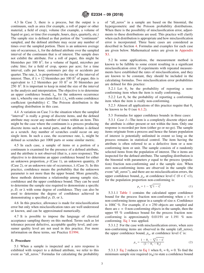
4.1 In Case 1, the sample is selected from a process or a very large population of interest. The population is essentially unlimited, and each item either has or has not the defined attribute. The population (process) has an unknown fraction of items p (long run average process non-conforming) having the attribute. The sample is a group of n discrete items selected at random from the process or population under consideration, and the attribute is not exhibited in the sample. The objective is to determine an upper confidence bound, pu, for the unknown fraction p whereby one can claim that p ≤ pu with some confidence coefficient (probability) C. The binomial distribution is the sampling distribution in this case.
4.2 In Case 2, a sample of n items is selected at random from a finite lot of N items. Like Case 1, each item either has or has not the defined attribute, and the population has an unknown number, D, of items having the attribute. The sample does not exhibit the attribute. The objective is to determine an upper confidence bound, Du, for the unknown number D, whereby one can claim that D ≤ Du with some confidence coefficient (probability) C. The hypergeometric distribution is the sampling distribution in this case.
4.3 In Case 3, there is a process, but the output is a continuum, such as area (for example, a roll of paper or other material, a field of crop), volume (for example, a volume of liquid or gas), or time (for example, hours, days, quarterly, etc.) The sample size is defined as that portion of the “continuum” sampled, and the defined attribute may occur any number of times over the sampled portion. There is an unknown average rate of occurrence, λ, for the defined attribute over the sampled interval of the continuum that is of interest. The sample does not exhibit the attribute. For a roll of paper, this might be blemishes per 100 ft2; for a volume of liquid, microbes per cubic litre; for a field of crop, spores per acre; for a time interval, ca...
SCOPE
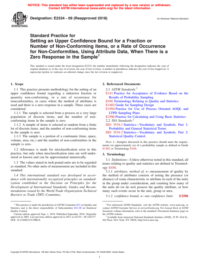
1.1 This practice presents methodology for the setting of an upper confidence bound regarding a unknown fraction or quantity non-conforming, or a rate of occurrence for nonconformities, in cases where the method of attributes is used and there is a zero response in a sample. Three cases are considered.
1.1.1 The sample is selected from a process or a very large population of discrete items, and the number of non-conforming items in the sample is zero.
1.1.2 A sample of items is selected at random from a finite lot of discrete items, and the number of non-conforming items in the sample is zero.
1.1.3 The sample is a portion of a continuum (time, space, volume, a...
General Information
Buy Standard
Standards Content (Sample)
NOTICE: This standard has either been superseded and replaced by a new version or withdrawn.
Contact ASTM International (www.astm.org) for the latest information
Designation: E2334 − 09 (Reapproved 2018) An American National Standard
Standard Practice for
Setting an Upper Confidence Bound for a Fraction or
Number of Non-Conforming items, or a Rate of Occurrence
for Non-Conformities, Using Attribute Data, When There is a
Zero Response in the Sample
This standard is issued under the fixed designation E2334; the number immediately following the designation indicates the year of
original adoption or, in the case of revision, the year of last revision. A number in parentheses indicates the year of last reapproval. A
superscript epsilon (´) indicates an editorial change since the last revision or reapproval.
1. Scope 2. Referenced Documents
1.1 This practice presents methodology for the setting of an 2.1 ASTM Standards:
upper confidence bound regarding a unknown fraction or E141 Practice for Acceptance of Evidence Based on the
quantity non-conforming, or a rate of occurrence for Results of Probability Sampling
nonconformities, in cases where the method of attributes is E456 Terminology Relating to Quality and Statistics
used and there is a zero response in a sample. Three cases are E1402 Guide for Sampling Design
considered. E1994 Practice for Use of Process Oriented AOQL and
1.1.1 The sample is selected from a process or a very large LTPD Sampling Plans
population of discrete items, and the number of non- E2586 Practice for Calculating and Using Basic Statistics
conforming items in the sample is zero. 2.2 ISO Standards:
1.1.2 A sample of items is selected at random from a finite ISO 3534-1 Statistics—Vocabulary and Symbols, Part 1:
lot of discrete items, and the number of non-conforming items Probability and General Statistical Terms
in the sample is zero. ISO 3534-2 Statistics—Vocabulary and Symbols, Part 2:
1.1.3 The sample is a portion of a continuum (time, space, Statistical Quality Control
volume, area, etc.) and the number of non-conformities in the
NOTE 1—Samples discussed in this practice should meet the require-
sample is zero.
ments (or approximately so) of a probability sample as defined in Guide
E1402 or Terminology E456.
1.2 Allowance is made for misclassification error in this
practice, but only when misclassification rates are well under-
3. Terminology
stood or known and can be approximated numerically.
3.1 Definitions—Unless otherwise noted in this standard, all
1.3 The values stated in inch-pound units are to be regarded
terms relating to quality and statistics are defined in Terminol-
as standard. No other units of measurement are included in this
ogy E456.
standard.
3.1.1 attributes, method of, n—measurement of quality by
1.4 This international standard was developed in accor- the method of attributes consists of noting the presence (or
dance with internationally recognized principles on standard-
absence) of some characteristic or attribute in each of the units
ization established in the Decision on Principles for the in the group under consideration, and counting how many of
Development of International Standards, Guides and Recom-
the units do (or do not) possess the quality attribute, or how
mendations issued by the World Trade Organization Technical many such events occur in the unit, group or area.
Barriers to Trade (TBT) Committee.
3.1.2 confidence bound, n—see confidence limit. E2586
1 2
This practice is under the jurisdiction of ASTM Committee E11 on Quality and For referenced ASTM Standards, visit the ASTM website, www.astm.org, or
Statistics and is the direct responsibility of Subcommittee E11.30 on Statistical contact ASTM Customer Service at service@astm.org. For Annual Book of ASTM
Quality Control. Standards volume information, refer to the standard’s Document Summary page on
Current edition approved Sept. 1, 2018. Published September 2018. Originally the ASTM website.
ɛ2 3
approved in 2003. Last previous edition approved in 2013 as E2334 – 09 (2013) . Available from American National Standards Institute (ANSI), 25 W. 43rd St.,
DOI: 10.1520/E2334-09R18. 4th Floor, New York, NY 10036, http://www.ansi.org.
Copyright © ASTM International, 100 Barr Harbor Drive, PO Box C700, West Conshohocken, PA 19428-2959. United States
E2334 − 09 (2018)
3.1.3 confidence coeffıcient, n—see confidence level. E2586 3.3.3 C —the confidence coefficient calculated that a pa-
d
rameter meets a certain requirement, that is, that p ≤ p , that
3.1.4 confidence interval, n—an interval estimate [L, U]
D ≤ D or that λ ≤ λ , when there is a zero response in the
0 0
with the statistics L and U as limits for the parameter θ and
sample.
with confidence level 1 – α, where Pr(L ≤ θ ≤ U) ≥ 1 – α.
3.3.4 D—the number of non-conforming items in a finite
E2586
population containing N items.
3.1.4.1 Discussion—The confidence level, 1 – α, reflects the
3.3.5 D —a specified value of D for which a researcher will
proportion of cases that the confidence interval [L, U] would
calculate a confidence coefficient for the statement, D ≤ D ,
contain or cover the true parameter value in a series of repeated 0
when there is a zero response in the sample.
random samples under identical conditions. Once L and U are
given values, the resulting confidence interval either does or
3.3.6 D —the upper confidence bound for the parameter D.
u
does not contain it. In this sense, “confidence” applies not to
3.3.7 N—the number of items in a finite population.
the particular interval but only to the long run proportion of
3.3.8 n—the sample size, that is, the number of items in a
cases when repeating the procedure many times.
sample.
3.1.5 confidence level, n—the value 1-α, of the probability
3.3.9 n —the sample size required.
R
associated with a confidence interval, often expressed as a
3.3.10 p—a process fraction non-conforming.
percentage. E2586
3.3.11 p —a specified value of p for which a researcher will
3.1.6 confidence limit, n—each of the limits, L and U, of a
calculate a confidence coefficient, for the statement p ≤ p ,
confidence interval, or the limit of a one-sided confidence
when there is a zero response in the sample.
interval. E2586
3.3.12 p —the upper confidence bound for the parameter p.
u
3.1.7 item, n—an object or quantity of material on which a
3.3.13 λ—the mean number of non-conformities (or events)
set of observations can be made.
over some area of interest for a Poisson process.
3.1.7.1 Discussion—As used in this practice, “set” denotes a
3.3.14 λ —a specific value of λ for which a researcher will
single variable (the defined attribute). The term “sampling
calculate a confidence coefficient for the statement, λ ≤ λ ,
unit” is also used to denote an “item” (see Practice E141).
when there is a zero response in the sample.
3.1.8 non-conforming item, n—an item containing at least
3.3.15 λ —the upper confidence bound for the parameter λ.
u
one non-conformity. ISO 3534-2
3.3.16 θ —the probability of classifying a conforming item
3.1.8.1 Discussion—The term “defective item” is also used
as non-conforming; or of finding a nonconformity where none
in this context.
exists.
3.1.9 non-conformity, n—the non-fulfillment of a specified
3.3.17 θ —the probability of classifying a non-conforming
requirement. ISO 3534-2
item as conforming; or of failing to find a non-conformity
3.1.9.1 Discussion—The term “defect” is also used in this
where one should have been found.
context.
4. Significance and Use
3.1.10 population, n—the totality of items or units of
material under consideration. E2586
4.1 In Case 1, the sample is selected from a process or a
very large population of interest. The population is essentially
3.1.11 probability sample, n—a sample in which the sam-
unlimited, and each item either has or has not the defined
pling units are selected by a chance process such that a
attribute. The population (process) has an unknown fraction of
specified probability of selection can be attached to each
items p (long run average process non-conforming) having the
possible sample that can be selected. E1402
attribute. The sample is a group of n discrete items selected at
3.1.12 sample, n—a group of observations or test results
random from the process or population under consideration,
taken from a larger collection of observations or test results,
and the attribute is not exhibited in the sample. The objective
which serves to provide information that may be used as a basis
is to determine an upper confidence bound, p , for the unknown
u
for making a decision concerning the larger collection. E2586
fraction p whereby one can claim that p ≤ p with some
u
confidence coefficient (probability) C. The binomial distribu-
3.2 Definitions of Terms Specific to This Standard:
tion is the sampling distribution in this case.
3.2.1 zero response, n—in the method of attributes, the
phrase used to denote that zero non-conforming items or zero 4.2 In Case 2, a sample of n items is selected at random
non-conformities were found (observed) in the item(s), unit, from a finite lot of N items. Like Case 1, each item either has
group, or area sampled. or has not the defined attribute, and the population has an
unknown number, D, of items having the attribute. The sample
3.3 Symbols:
does not exhibit the attribute. The objective is to determine an
3.3.1 A—the assurance index, as a percent or a probability
upper confidence bound, D , for the unknown number D,
u
value.
whereby one can claim that D ≤ D with some confidence
u
3.3.2 C—confidence coefficient as a percent or as a prob- coefficient (probability) C. The hypergeometric distribution is
ability value. the sampling distribution in this case.
E2334 − 09 (2018)
4.3 In Case 3, there is a process, but the output is a of “all_zeros” in a sample are based on the binomial, the
continuum, such as area (for example, a roll of paper or other hypergeometric and the Poisson probability distributions.
material, a field of crop), volume (for example, a volume of When there is the possibility of misclassification error, adjust-
liquid or gas), or time (for example, hours, days, quarterly, etc.) ments to these distributions are used. This practice will clarify
The sample size is defined as that portion of the “continuum” when each distribution is appropriate and how misclassification
sampled, and the defined attribute may occur any number of error is incorporated. Three basic cases are considered as
times over the sampled portion. There is an unknown average described in Section 4. Formulas and examples for each case
rate of occurrence, λ, for the defined attribute over the sampled are given below. Mathematical notes are given in Appendix
interval of the continuum that is of interest. The sample does X1.
not exhibit the attribute. For a roll of paper, this might be
5.2 In some applications, the measurement method is
blemishes per 100 ft ; for a volume of liquid, microbes per
known to be fallible to some extent resulting in a significant
cubic litre; for a field of crop, spores per acre; for a time
misclassification error. If experiments with repeated measure-
interval, calls per hour, customers per day or accidents per
ments have established the rates of misclassification, and they
quarter. The rate, λ, is proportional to the size of the interval of
are known to be constant, they should be included in the
interest. Thus, if λ = 12 blemishes per 100 ft of paper, this is
calculating formulas. Two misclassification error probabilities
equivalent to 1.2 blemishes per 10 ft or 30 blemishes per
are defined for this practice:
250 ft . It is important to keep in mind the size of the interval
5.2.1 Let θ be the probability of reporting a non-
in the analysis and interpretation. The objective is to determine
conforming item when the item is really conforming.
an upper confidence bound, λ , for the unknown occurrence
u
5.2.2 Let θ be the probability of reporting a conforming
rate λ, whereby one can claim that λ ≤ λ with some confidence
u
item when the item is really non-conforming.
coefficient (probability) C. The Poisson distribution is the
5.2.3 Almost all applications of this practice require that θ
sampling distribution in this case.
be known to be 0 (see 6.1.2).
4.4 A variation on Case 3 is the situation where the sampled
5.3 Formulas for upper confidence bounds in three cases:
“interval” is really a group of discrete items, and the defined
attribute may occur any number of times within an item. This 5.3.1 Case 1—The item is a completely discrete object and
the attribute is either present or not within the item. Only one
might be the case where the continuum is a process producing
discrete items such as metal parts, and the attribute is defined response is recorded per item (either go or no-go). The sample
items originate from a process and hence the future population
as a scratch. Any number of scratches could occur on any
single item. In such a case, the occurrence rate, λ, might be of interest is potentially unlimited in extent so long as the
process remains in statistical control. The item having the
defined as scratches per 1000 parts or some similar metric.
attribute is often referred to as a defective item or a non-
4.5 In each case, a sample of items or a portion of a
conforming item or unit. The sample consists of n randomly
continuum is examined for the presence of a defined attribute,
selected items from the population of interest. The n items are
and the attribute is not observed (that is, a zero response). The
inspected for the defined attribute. The sampling distribution is
objective is to determine an upper confidence bound for either
the binomial with parameters p equal to the process (popula-
an unknown proportion, p (Case 1), an unknown quantity, D
tion) fraction non-conforming and n the sample size. When
(Case 2), or an unknown rate of occurrence, λ (Case 3). In this
zero non-conforming items are observed in the sample (the
practice, confidence means the probability that the unknown
event “all_zeros”), and there are no misclassification errors, the
parameter is not more than the upper bound. More generally,
upper confidence bound, p , at confidence level C (0 < C <1),
u
these methods determine a relationship among sample size,
for the population proportion non-conforming is:
confidence and the upper confidence bound. They can be used
n
to determine the sample size required to demonstrate a specific
p 5 1 2 =1 2 C (1)
u
p, D, or λ with some degree of confidence. They can also be
5.3.1.1 Table 1 contains the calculated upper confidence
used to determine the degree of confidence achieved in
bound for the process fraction non-conforming when x = 0
demonstrating a specified p, D, or λ.
non-conforming items appear in a sample of size n. Confidence
4.6 In this practice, allowanc
...
This document is not an ASTM standard and is intended only to provide the user of an ASTM standard an indication of what changes have been made to the previous version. Because
it may not be technically possible to adequately depict all changes accurately, ASTM recommends that users consult prior editions as appropriate. In all cases only the current version
of the standard as published by ASTM is to be considered the official document.
´2
Designation: E2334 − 09 (Reapproved 2013) E2334 − 09 (Reapproved 2018)An American National Standard
Standard Practice for
Setting an Upper Confidence Bound Forfor a Fraction or
Number of Non-Conforming items, or a Rate of Occurrence
for Non-conformities,Non-Conformities, Using Attribute
Data, When There is a Zero Response in the Sample
This standard is issued under the fixed designation E2334; the number immediately following the designation indicates the year of
original adoption or, in the case of revision, the year of last revision. A number in parentheses indicates the year of last reapproval. A
superscript epsilon (´) indicates an editorial change since the last revision or reapproval.
ε NOTE—Section 3 was editorially corrected in August 2013.
ε NOTE—Terms were editorially corrected in April 2016.
1. Scope
1.1 This practice presents methodology for the setting of an upper confidence bound regarding a unknown fraction or quantity
non-conforming, or a rate of occurrence for nonconformities, in cases where the method of attributes is used and there is a zero
response in a sample. Three cases are considered.
1.1.1 The sample is selected from a process or a very large population of discrete items, and the number of non-conforming
items in the sample is zero.
1.1.2 A sample of items is selected at random from a finite lot of discrete items, and the number of non-conforming items in
the sample is zero.
1.1.3 The sample is a portion of a continuum (time, space, volume, area, etc.) and the number of non-conformities in the sample
is zero.
1.2 Allowance is made for misclassification error in this standard,practice, but only when misclassification rates are well
understood or known and can be approximated numerically.
1.3 The values stated in inch-pound units are to be regarded as standard. No other units of measurement are included in this
standard.
1.4 This international standard was developed in accordance with internationally recognized principles on standardization
established in the Decision on Principles for the Development of International Standards, Guides and Recommendations issued
by the World Trade Organization Technical Barriers to Trade (TBT) Committee.
2. Referenced Documents
2.1 ASTM Standards:
E141 Practice for Acceptance of Evidence Based on the Results of Probability Sampling
E456 Terminology Relating to Quality and Statistics
E1402 Guide for Sampling Design
E1994 Practice for Use of Process Oriented AOQL and LTPD Sampling Plans
E2586 Practice for Calculating and Using Basic Statistics
2.2 ISO Standards:
ISO 3534-1 Statistics—Vocabulary and Symbols, Part 1: Probability and General Statistical Terms
ISO 3534-2 Statistics—Vocabulary and Symbols, Part 2: Statistical Quality Control
NOTE 1—Samples discussed in this standardpractice should meet the requirements (or approximately so) of a probability sample as defined in
TerminologiesGuide E1402 or Terminology E456.
This practice is under the jurisdiction of ASTM Committee E11 on Quality and Statistics and is the direct responsibility of Subcommittee E11.30 on Statistical Quality
Control.
Current edition approved April 1, 2013Sept. 1, 2018. Published April 2013September 2018. Originally approved in 2003. Last previous edition approved in 20092013 as
ɛ2
E2334 – 09.E2334 – 09 (2013) . DOI: 10.1520/E2334-09R13E02.10.1520/E2334-09R18.
For referenced ASTM Standards, visit the ASTM website, www.astm.org, or contact ASTM Customer Service at service@astm.org. For Annual Book of ASTM Standards
volume information, refer to thestandard’s the standard’s Document Summary page on the ASTM website.
Available from American National Standards Institute (ANSI), 25 W. 43rd St., 4th Floor, New York, NY 10036, http://www.ansi.org.
Copyright © ASTM International, 100 Barr Harbor Drive, PO Box C700, West Conshohocken, PA 19428-2959. United States
E2334 − 09 (2018)
3. Terminology
3.1 Definitions—Unless otherwise noted in this standard, all terms relating to quality and statistics are defined in Terminology
E456.
3.1.1 attributes, method of, n—measurement of quality by the method of attributes consists of noting the presence (or absence)
of some characteristic or attribute in each of the units in the group under consideration, and counting how many of the units do
(or do not) possess the quality attribute, or how many such events occur in the unit, group or area.
3.1.2 confidence bound, n—see confidence limit. E2586
3.1.3 confidence coeffıcient, n—see confidence level. E2586
3.1.4 confidence interval, n—an interval estimate [L, U] with the statistics L and U as limits for the parameter θ and with
confidence level 1 – α, where Pr(L ≤ θ ≤ U) ≥ 1 – α. E2586
3.1.4.1 Discussion—
The confidence level, 1 – α, reflects the proportion of cases that the confidence interval [L, U] would contain or cover the true
parameter value in a series of repeated random samples under identical conditions. Once L and U are given values, the resulting
confidence interval either does or does not contain it. In this sense "confidence"sense, “confidence” applies not to the particular
interval but only to the long run proportion of cases when repeating the procedure many times.
3.1.5 confidence level, n—the value 1-α, of the probability associated with a confidence interval, often expressed as a
percentage. E2586
3.1.6 confidence limit, n—each of the limits, L and U, of a confidence interval, or the limit of a one-sided confidence interval.
E2586
3.1.7 item, n—an object or quantity of material on which a set of observations can be made.
3.1.7.1 Discussion—
As used in this standard,practice, “set” denotes a single variable (the defined attribute). The term “sampling unit” is also used to
denote an “item” (see Practice E141).
3.1.8 non-conforming item, n—an item containing at least one non-conformity. ISO 3534-2
3.1.8.1 Discussion—
The term “defective item” is also used in this context.
3.1.9 non-conformity, n—the non-fulfillment of a specified requirement. ISO 3534-2
3.1.9.1 Discussion—
The term “defect” is also used in this context.
3.1.10 population, n—the totality of items or units of material under consideration. E2586
3.1.11 probability sample, n—a sample in which the sampling units are selected by a chance process such that a specified
probability of selection can be attached to each possible sample that can be selected. E1402
3.1.12 sample, n—a group of observations or test results taken from a larger collection of observations or test results, which
serves to provide information that may be used as a basis for making a decision concerning the larger collection. E2586
3.2 Definitions of Terms Specific to This Standard:
3.2.1 zero response, n—in the method of attributes, the phrase used to denote that zero non-conforming items or zero
non-conformities were found (observed) in the item(s), unit, group, or area sampled.
3.3 Symbols:
3.3.1 A—the assurance index, as a percent or a probability value.
3.3.2 C—confidence coefficient as a percent or as a probability value.
3.3.3 C —the confidence coefficient calculated that a parameter meets a certain requirement, that is, that p ≤ p , that D ≤ ≤ D
d 0 0
or that λ ≤ λ , when there is a zero response in the sample.
3.3.4 D—the number of non-conforming items in a finite population containing N items.
3.3.5 D —a specified value of D for which a researcher will calculate a confidence coefficient for the statement, D ≤ D , when
0 0
there is a zero response in the sample.
E2334 − 09 (2018)
3.3.6 D —the upper confidence bound for the parameter D.
u
3.3.7 N—the number of items in a finite population.
3.3.8 n—the sample size, that is, the number of items in a sample.
3.3.9 n —the sample size required.
R
3.3.10 p—a process fraction non-conforming.
3.3.11 p —a specified value of p for which a researcher will calculate a confidence coefficient, for the statement p ≤ p , when
0 0
there is a zero response in the sample.
3.3.12 p —the upper confidence bound for the parameter p.
u
3.3.13 λ—the mean number of non-conformities (or events) over some area of interest for a Poisson process.
3.3.14 λ —a specific value of λ for which a researcher will calculate a confidence coefficient for the statement, λ ≤ λ , when
0 0
there is a zero response in the sample.
3.3.15 λ —the upper confidence bound for the parameter λ.
u
3.3.16 θ —the probability of classifying a conforming item as non-conforming; or of finding a nonconformity where none
exists.
3.3.17 θ —the probability of classifying a non-conforming item as conforming; or of failing to find a non-conformity where one
should have been found.
4. Significance and Use
4.1 In Case 1, the sample is selected from a process or a very large population of interest. The population is essentially
unlimited, and each item either has or has not the defined attribute. The population (process) has an unknown fraction of items p
(long run average process non-conforming) having the attribute. The sample is a group of n discrete items selected at random from
the process or population under consideration, and the attribute is not exhibited in the sample. The objective is to determine an
upper confidence bound, p , for the unknown fraction p whereby one can claim that p ≤ p with some confidence coefficient
u u
(probability) C. The binomial distribution is the sampling distribution in this case.
4.2 In Case 2, a sample of n items is selected at random from a finite lot of N items. Like Case 1, each item either has or has
not the defined attribute, and the population has an unknown number, D, of items having the attribute. The sample does not exhibit
the attribute. The objective is to determine an upper confidence bound, D , for the unknown number D, whereby one can claim
u
that D ≤ D with some confidence coefficient (probability) C. The hypergeometric distribution is the sampling distribution in this
u
case.
4.3 In Case 3, there is a process, but the output is a continuum, such as area (for example, a roll of paper or other material, a
field of crop), volume (for example, a volume of liquid or gas), or time (for example, hours, days, quarterly, etc.) The sample size
is defined as that portion of the “continuum” sampled, and the defined attribute may occur any number of times over the sampled
portion. There is an unknown average rate of occurrence, λ, for the defined attribute over the sampled interval of the continuum
that is of interest. The sample does not exhibit the attribute. For a roll of paper, this might be blemishes per 100 ft ; for a volume
of liquid, microbes per cubic litre; for a field of crop, spores per acre; for a time interval, calls per hour, customers per day or
accidents per quarter. The rate, λ, is proportional to the size of the interval of interest. Thus, if λ = 12 blemishes per 100 ft of paper,
2 2
this is equivalent to 1.2 blemishes per 10 ft or 30 blemishes per 250 ft250 ft . It is important to keep in mind the size of the
interval in the analysis and interpretation. The objective is to determine an upper confidence bound, λ , for the unknown occurrence
u
rate λ, whereby one can claim that λ ≤ λ with some confidence coefficient (probability) C. The Poisson distribution is the sampling
u
distribution in this case.
4.4 A variation on Case 3 is the situation where the sampled “interval” is really a group of discrete items, and the defined
attribute may occur any number of times within an item. This might be the case where the continuum is a process producing
discrete items such as metal parts, and the attribute is defined as a scratch. Any number of scratches could occur on any single item.
In such a case, the occurrence rate, λ, might be defined as scratches per 1000 parts or some similar metric.
4.5 In each case, a sample of items or a portion of a continuum is examined for the presence of a defined attribute, and the
attribute is not observed (that is, a zero response). The objective is to determine an upper confidence bound for either an unknown
proportion, p (Case 1), an unknown quantity, D (Case 2), or an unknown rate of occurrence, λ (Case 3). In this standard,practice,
confidence means the probability that the unknown parameter is not more than the upper bound. More generally, these methods
determine a relationship among sample size, confidence and the upper confidence bound. They can be used to determine the sample
size required to demonstrate a specific p,D, or λ with some degree of confidence. They can also be used to determine the degree
of confidence achieved in demonstrating a specified p,D, or λ.
4.6 In this standardpractice, allowance is made for misclassification error but only when misclassification rates are well
understood or known, and can be approximated numerically.
E2334 − 09 (2018)
4.7 It is possible to impose the language of classical acceptance sampling theory on this method. Terms such as Lot Tolerance
Percent Defective, Acceptable Quality Level, Consumer Quality Level lot tolerance percent defective, acceptable quality level, and
consumer quality level are not used in this standard.practice. For more information on these terms, see Practice E1994.
5. Procedure
5.1 When a sample is inspected and a zero response is exhibited with respect to a defined attribute, we refer to this event as
“all_zeros.” Formulas for calculating the probability of “all_zeros” in a sample are based on the binomial, the hypergeometric and
the Poisson probability distributions. When there is the possibility of misclassification error, adjustments to these distributions are
used. This practice will clarify when each distribution is appropriate and how misclassification error is incorporated. Three basic
cases are considered as described in Section 4. Formulas and examples for each case are given below. Mathematical notes are given
in Appendix X1.
5.2 In some applications, the measurement method is known to be fallible to some extent resulting in a significant
misclassification error. If experiments with repeated measurements have established the rates of misclassification, and they are
known to be constant, they should be included in the calculating formulas. Two misclassification error probabilities are defined for
this practice:
5.2.1 Let θ be the probability of reporting a non-conforming item when the item is really conforming.
5.2.2 Let θ be the probability of reporting a conforming item when the item is really non-conforming.
5.2.3 Almost all applications of this s
...
Questions, Comments and Discussion
Ask us and Technical Secretary will try to provide an answer. You can facilitate discussion about the standard in here.