ASTM G166-00(2020)

Standard Guide for Statistical Analysis of Service Life Data

SIGNIFICANCE AND USE
4.1 Service life test data often show different distribution shapes than many other types of data. This is due to the effects of measurement error (typically normally distributed), combined with those unique effects which skew service life data towards early failure (infant mortality failures) or late failure times (aging or wear-out failures) Applications of the principles in this guide can be helpful in allowing investigators to interpret such data.
Note 2: Service life or reliability data analysis packages are becoming more readily available in standard or common computer software packages. This puts data reduction and analyses more readily into the hands of a growing number of investigators.
SCOPE
1.1 This guide presents briefly some generally accepted methods of statistical analyses which are useful in the interpretation of service life data. It is intended to produce a common terminology as well as developing a common methodology and quantitative expressions relating to service life estimation.  
1.2 This guide does not cover detailed derivations, or special cases, but rather covers a range of approaches which have found application in service life data analyses.  
1.3 Only those statistical methods that have found wide acceptance in service life data analyses have been considered in this guide.  
1.4 The Weibull life distribution model is emphasized in this guide and example calculations of situations commonly encountered in analysis of service life data are covered in detail.  
1.5 The choice and use of a particular life distribution model should be based primarily on how well it fits the data and whether it leads to reasonable projections when extrapolating beyond the range of data. Further justification for selecting a model should be based on theoretical considerations.  
1.6 This international standard was developed in accordance with internationally recognized principles on standardization established in the Decision on Principles for the Development of International Standards, Guides and Recommendations issued by the World Trade Organization Technical Barriers to Trade (TBT) Committee.

General Information

• Status: Published
• Publication Date: 14-Feb-2020
• ICS: 13.020.60 - Product life-cycles
• Technical Committee: G03 - Weathering and Durability
• Drafting Committee: G03.08 - Service Life Prediction

Relations

• Replaces: ASTM G166-00(2011) - Standard Guide for Statistical Analysis of Service Life Data
• Effective Date: 15-Feb-2020
• Refers: ASTM G169-01(2008)e1 - Standard Guide for Application of Basic Statistical Methods to Weathering Tests
• Effective Date: 01-Jun-2008
• Refers: ASTM G169-01 - Standard Guide for Application of Basic Statistical Methods to Weathering Tests
• Effective Date: 10-Jan-2001
• Referred By: ASTM G141-09(2021) - Standard Guide for Addressing Variability in Exposure Testing of Nonmetallic Materials
• Effective Date: 15-Feb-2020
• Referred By: ASTM G172-19 - Standard Guide for Statistical Analysis of Accelerated Service Life Data
• Effective Date: 15-Feb-2020

Overview

ASTM G166-00(2020) - Standard Guide for Statistical Analysis of Service Life Data provides a comprehensive framework for analyzing the service life or reliability of materials and products using statistical methods. Developed by ASTM International, this standard is designed to create common terminology and methodologies for the interpretation of service life data. It emphasizes practical tools for data analysis and model selection, with a detailed focus on the Weibull life distribution model.

Many service life test datasets exhibit unique characteristics, such as non-normal distributions, caused by early or late failures (commonly described as "infant mortality" or "wear-out" failures). This guide assists investigators in properly analyzing these patterns, selecting appropriate statistical models, and making informed life estimations.

Key Topics

• Common Methodologies: Presents generally accepted methods for analyzing service life data, focusing on approaches with broad industry acceptance.
• Weibull Distribution Focus: Detailed guidance on using the Weibull model, highly valued for its flexibility in representing various failure behaviors.
• Terminology Standardization: Defines terms such as service life, beginning and end of life, probability of failure, reliability, and parameter estimation techniques.
• Model Selection Principles: Guidance on selecting the most appropriate life distribution model based on fit to observed data and theoretical soundness.
• Complete and Incomplete Data Handling: Outlines best practices in dealing with complete datasets (all specimens failed) and incomplete datasets (right/left censored or multiply censored data).
• Use of Modern Software: Notes the increasing availability of statistical and reliability analysis tools in commonly used software, making such analyses accessible to more investigators.

Applications

This ASTM standard has broad applications across industries where product longevity, reliability, and maintenance scheduling are critical. Typical usage scenarios include:

• Product Quality Assurance: Supporting evidence-based warranty and maintenance interval decisions for consumer products, automotive parts, electronics, and industrial equipment.
• Accelerated Life Testing: Estimating expected service life under normal and accelerated conditions for predictive maintenance and risk assessment.
• Material Durability Assessment: Analyzing the degradation or failure of construction materials, coatings, and polymers exposed to environmental or operational stresses.
• Reliability Engineering: Providing the statistical backbone for reliability predictions, root cause analysis, and the development of maintenance strategies.
• R&D and Product Design: Assisting researchers and engineers in understanding failure mechanisms and improving the design of longer-lasting products.
• Regulatory Compliance: Adhering to best practices consistent with internationally recognized standards on statistical analysis and service life estimation.

By applying statistical analysis in line with ASTM G166, organizations can better predict failure rates, establish realistic service intervals, and optimize resource allocation for testing, maintenance, and recalls.

Related Standards

Several other ASTM and international standards complement the practices described in ASTM G166-00(2020):

• ASTM G169: Guide for Application of Basic Statistical Methods to Weathering Tests
• ASTM E2281: Standard Practice for Specimen Preparation and Data Analysis for Interlaboratory Study Involving Outlier Treatment and Performance Assessment
• ISO 3534-1: Statistics - Vocabulary and symbols
• IEC 61649: Weibull analysis standard for reliability testing

These documents provide additional guidance on statistical techniques, data handling, and specific applications in material durability and failure analysis.

Keywords: ASTM G166, service life data, statistical analysis, reliability, Weibull distribution, life estimation, censored data, durability testing, product failure, ASTM standard.

Standards Content (Sample)

This international standard was developed in accordance with internationally recognized principles on standardization established in the Decision on Principles for the
Development of International Standards, Guides and Recommendations issued by the World Trade Organization Technical Barriers to Trade (TBT) Committee.
Designation: G166 − 00 (Reapproved 2020)
Standard Guide for
Statistical Analysis of Service Life Data
This standard is issued under the fixed designation G166; the number immediately following the designation indicates the year of
original adoption or, in the case of revision, the year of last revision.Anumber in parentheses indicates the year of last reapproval.A
superscript epsilon (´) indicates an editorial change since the last revision or reapproval.
1. Scope 3. Terminology
1.1 This guide presents briefly some generally accepted 3.1 Definitions:
methods of statistical analyses which are useful in the inter-
3.1.1 material property—customarily, service life is consid-
pretation of service life data. It is intended to produce a
ered to be the period of time during which a system meets
common terminology as well as developing a common meth-
critical specifications. Correct measurements are essential to
odology and quantitative expressions relating to service life
producing meaningful and accurate service life estimates.
estimation.
3.1.1.1 Discussion—There exists many ASTM recognized
1.2 This guide does not cover detailed derivations, or
and standardized measurement procedures for determining
special cases, but rather covers a range of approaches which
material properties. As these practices have been developed
have found application in service life data analyses.
withincommitteeswithappropriateexpertise,nofurtherelabo-
1.3 Only those statistical methods that have found wide
ration will be provided.
acceptance in service life data analyses have been considered
3.1.2 beginning of life—this is usually determined to be the
in this guide.
time of manufacture. Exceptions may include time of delivery
1.4 TheWeibulllifedistributionmodelisemphasizedinthis
to the end user or installation into field service.
guide and example calculations of situations commonly en-
3.1.3 end of life—Occasionally this is simple and obvious
countered in analysis of service life data are covered in detail.
such as the breaking of a chain or burning out of a light bulb
1.5 Thechoiceanduseofaparticularlifedistributionmodel
filament. In other instances, the end of life may not be so
should be based primarily on how well it fits the data and
catastrophic and free from argument. Examples may include
whether it leads to reasonable projections when extrapolating
fading, yellowing, cracking, crazing, etc. Such cases need
beyond the range of data. Further justification for selecting a
quantitative measurements and agreement between evaluator
model should be based on theoretical considerations.
anduserastotheprecisedefinitionoffailure.Itisalsopossible
1.6 This international standard was developed in accor-
to model more than one failure mode for the same specimen.
dance with internationally recognized principles on standard-
(Forexample,thetimetoproduceagivenamountofyellowing
ization established in the Decision on Principles for the
may be measured on the same specimen that is also tested for
Development of International Standards, Guides and Recom-
cracking.)
mendations issued by the World Trade Organization Technical
Barriers to Trade (TBT) Committee.
3.1.4 F(t)—The probability that a random unit drawn from
the population will fail by time (t). Also F(t) = the decimal
2. Referenced Documents
fractionofunitsinthepopulationthatwillfailbytime (t).The
decimal fraction multiplied by 100 is numerically equal to the
2.1 ASTM Standards:
percent failure by time (t).
G169Guide for Application of Basic Statistical Methods to
Weathering Tests
3.1.5 R(t)—The probability that a random unit drawn from
the population will survive at least until time (t). Also R(t) =
the fraction of units in the population that will survive at least
This guide is under the jurisdiction of ASTM Committee G03 on Weathering
until time (t)
and Durability and is the direct responsibility of Subcommittee G03.08 on Service
Life Prediction.
R t 51 2 F t (1)
~ ! ~ !
Current edition approved Feb. 15, 2020. Published March 2020. Originally
approvedin2000.Lastpreviouseditionapprovedin2011asG166–00(2011).DOI:
3.1.6 pdf—theprobabilitydensityfunction(pdf),denotedby
10.1520/G0166-00R20.
f(t),equalstheprobabilityoffailurebetweenanytwopointsof
For referenced ASTM standards, visit the ASTM website, www.astm.org, or
dF ~t!
contact ASTM Customer Service at [e-mail]. For Annual Book of ASTM
time t(1) and t(2). Mathematically f t 5 . For the normal
~ !
dt
Standards volume information, refer to the standard’s Document Summary page on
the ASTM website. distribution, the pdf is the “bell shape” curve.
Copyright © ASTM International, 100 Barr Harbor Drive, PO Box C700, West Conshohocken, PA 19428-2959. United States
G166 − 00 (2020)
3.1.7 cdf—the cumulative distribution function (cdf), de- consideredtobetimecensored.Thisisalsoreferredtoasright
noted by F(t), represents the probability of failure (or the censored or type I censoring. Graphical solutions can still be
population fraction failing) by time = (t). See section 3.1.4. used for parameter estimation. At least ten observed failures
should be used for estimating parameters (for example slope
3.1.8 weibull distribution—For the purposes of this guide,
and intercept).
the Weibull distribution is represented by the equation:
3.1.10.2 specimen censored—Specimens that were still sur-
t b
2S D
F~t! 51 2 e c (2)
viving when the test was terminated after a set number of
failures are considered to be specimen censored. This is
where:
anothercaseofrightcensoredortypeIcensoring.See3.1.10.1
F(t) = defined in paragraph 3.1.4
3.1.10.3 Multiply Censored—Specimens that were removed
t = units of time used for service life
priortotheendofthetestwithoutfailingarereferredtoasleft
c = scale parameter
b = shape parameter
censored or type II censored. Examples would include speci-
mens that were lost, dropped, mishandled, damaged or broken
3.1.8.1 The shape parameter (b), section 3.1.6, is so called
duetostressesnotpartofthetest.Adjustmentsoffailureorder
because this parameter determines the overall shape of the
can be made for those specimens actually failed.
curve. Examples of the effect of this parameter on the distri-
bution curve are shown in Fig. 1, section 5.3.
4. Significance and Use
3.1.8.2 The scale parameter (c), section 3.1.6, is so called
4.1 Service life test data often show different distribution
because it positions the distribution along the scale of the time
shapes than many other types of data.This is due to the effects
axis. It is equal to the time for 63.2% failure.
of measurement error (typically normally distributed), com-
NOTE 1—This is arrived at by allowing t to equal c in the above
bined with those unique effects which skew service life data
−1
expression.ThisthenreducestoFailureProbability=1−e ,whichfurther
towards early failure (infant mortality failures) or late failure
reduces to equal 1−0.368 or .632.
times (aging or wear-out failures) Applications of the prin-
3.1.9 completedata—Acompletedatasetisonewhereallof
ciples in this guide can be helpful in allowing investigators to
thespecimensplacedontestfailbytheendoftheallocatedtest
interpret such data.
time.
NOTE2—Servicelifeorreliabilitydataanalysispackagesarebecoming
3.1.10 Incomplete data—An incomplete data set is one
more readily available in standard or common computer software pack-
where (a) there are some specimens that are still surviving at
ages.Thisputsdatareductionandanalysesmorereadilyintothehandsof
the expiration of the allowed test time, (b) where one or more
a growing number of investigators.
specimens is removed from the test prior to expiration of the
5. Data Analysis
allowedtesttime.Theshapeandscaleparametersoftheabove
distributions may be estimated even if some of the test
5.1 In the determinations of service life, a variety of factors
specimensdidnotfail.Therearethreedistinctcaseswherethis
act to produce deviations from the expected values. These
might occur.
factors may be of a purely random nature and act to either
3.1.10.1 Time censored—Specimens that were still surviv- increaseordecreaseservicelifedependingonthemagnitudeof
ing when the test was terminated after elapse of a set time are the factor. The purity of a lubricant is an example of one such
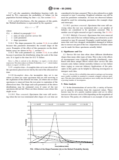
FIG. 1 Effect of the Shape Parameter (b) on the Weibull Probability Density
G166 − 00 (2020)
factor. An oil clean and free of abrasives and corrosive flexing,cracks,crackangle,numberofflexes,etc.Performance
materials would be expected to prolong the service life of a eventually degrades to the defined end of life.
5.3.1 Thereareseveralconvenientfeaturesofthelognormal
moving part subject to wear. A fouled contaminated oil might
prove to be harmful and thereby shorten service life. Purely distribution. First, there is essentially no new mathematics to
introduce into the analysis of this distribution beyond those of
randomvariationinanagingfactorthatcaneitherhelporharm
thenormaldistribution.Asimplelogarithmictransformationof
a service life might lead a normal, or gaussian, distribution.
data converts lognormal distributed data into a normal distri-
Such distributions are symmetrical about a central tendency,
bution.Allofthetables,graphs,analysisroutinesetc.maythen
usually the mean.
be used to describe the transformed function. One note of
5.1.1 Some non-random factors act to skew service life
caution is that the shape parameter σ is symmetrical in its
distributions. Defects are generally thought of as factors that
logarithmicformandnon-symmetricalinitsnaturalform.(For
can only decrease service life. Thin spots in protective
example, x¯=1 6 .2σ in logarithmic form translates to 10 +5.8
coatings, nicks in extruded wires, chemical contamination in
and −3.7 in natural form.)
thin metallic films are examples of such defects that can cause
5.3.2 As there is no symmetrical restriction, the shape of
an overall failure even through the bulk of the material is far
thisfunctionmaybeabetterfitthanthenormaldistributionfor
from failure. These factors skew the service life distribution
the service life distributions of the material being investigated.
towards early failure times.
5.4 Weibull Distribution—While the Swedish Professor
5.1.2 Factors that skew service life towards the high side
Waloddi Weibull was not the first to use this expression, his
also exist. Preventive maintenance, high quality raw materials,
paper, A Statistical Distribution of Wide Applicability pub-
reduced impurities, and inhibitors or other additives are such
lished in 1951 did much to draw attention to this exponential
factors. These factors produce life time distributions shifted
function. The simplicity of formula given in (1), hides its
towardsthelongtermandarethosetypicallyfoundinproducts
extreme flexibility to model service life distributions.
having been produced a relatively long period of time.
5.4.1 The Weibull distribution owes its flexibility to the
5.1.3 Establishing a description of the distribution of fre-
“shape” parameter. The shape of this distribution is dependent
quency (or probability) of failure versus time in service is the
on the value of b. If b is less than 1, the Weibull distribution
objective of this guide. Determination of the shape of this
modelsfailuretimeshavingadecreasingfailurerate.Thetimes
distribution as well as its position along the time scale axis are
betweenfailuresincreasewithexposuretime.Ifb=1,thenthe
the principle criteria for estimating service life.
Weibull models failure times having constant failure rate. If b
> 1 it models failure times having an increasing failure rate, if
5.2 Normal (Gaussian) Distribution—The characteristic of
b = 2, then Weibull exactly duplicates the Rayleigh
the normal, or Gaussian distribution is a symmetrical bell
distribution, as b approaches 2.5 it very closely approximates
shaped curve centered on the mean of this distribution. The
the lognormal distribution, as b approaches 3. the Weibull
meanrepresentsthetimefor50%failure.Thismaybedefined
expression models the normal distribution and as b grows
as either the time when one can expect 50% of the entire
beyond 4, the Weibull expression models distributions skewed
population to fail or the probability of an individual item to
towards long failure times. See Fig. 1 for examples of
fail.The“scale”ofthenormalcurveisthemeanvalue(x¯),and
distributions with different shape parameters.
the shape of this curve is established by the standard deviation
5.4.2 The Weibull distribution is most appropriate when
value (σ).
therearemanypossiblesiteswherefailuremightoccurandthe
5.2.1 The normal distribution has found widespread use in
system fails upon the occurrence of the first site failure. An
describing many naturally occurring distributions. Its first
example commonly used for this type of situation is a chain
known description by Carl Gauss showed its applicability to
failing when only one link separates.All of the sites, or links,
measurement error. Its applications are widely known and
areequallyatrisk,yetoneisallthatisrequiredfortotalfailure.
numerous texts produce exhaustive tables and descriptions of
5.5 Exponential Distribution—This distribution is a special
this function.
case of the Weibull. It is useful to simplify calculations
5.2.2 Widespread use should not be confused with justifi-
involving periods of service life that are subject to random
cation for its application to service life data. Use of analysis
failures. These would include random defects but not include
techniques developed for normal distribution on data distrib-
wear-out or burn-in periods.
uted in a non-normal manner can lead to grossly erroneous
conclusions. As described in Section 5, many service life
6. Parameter Estimation
distributions are skewed towards either early life or late life.
6.1 Weibull data analysis functions are not uncommon but
The confinement to a symmetrical shape is the principal
not yet found on all data analysis packages. Fortunately, the
shortcoming of the normal distribution for service life appli-
expression is simple enough so that parameter estimation may
cations. This may lead to situations where even negative
lifetimes are predicted.
Mann,N.R.etal., Methods for StatisticalAnalysis of Reliability and Life Data,
5.3 Lognormal Distribution—This distribution has shown
Wiley, New York 1974 and Gnedenko, B.V. et al, Mathematical Methods of
application when the specimen fails due to a multiplicative
Reliability Theory, Academic Press, New York 1969.
process that degrades performance over time. Metal fatigue is 4
Weibull, W., “A statistical distribution of wide applicability ,” J. Appl. Mech.,
one example. Degradation is a function of the amount of 18, 1951, pp 293–2
...